---
title: "Introduction to influential"
subtitle: "Network influence analysis, centrality assessment, and experimental feature prioritization"
author: '`r paste("Adrian Salavaty",strftime(Sys.time(),format="%d-%b-%Y"))`'
output:
rmarkdown::html_vignette:
css: influentialVignette.css
toc: true
toc_depth: 3
df_print: paged
number_sections: true
vignette: >
%\VignetteIndexEntry{Introduction to influential}
%\VignetteEngine{knitr::rmarkdown}
%\VignetteEncoding{UTF-8}
---
```{r, include = FALSE}
knitr::opts_chunk$set(
collapse = TRUE,
comment = "#>",
fig.width = 7,
fig.height = 5.4,
out.width = "92%"
)
options(tibble.print_min = 4L, tibble.print_max = 4L)
options(width = 95)
options(rmarkdown.html_vignette.check_title = FALSE)
set.seed(60)
```
```{r, echo=FALSE}
spaces <- function (n) {
paste(rep(" ", n), collapse = "")
}
```
# Overview
`influential` is an R package for identifying influential nodes in networks and for classifying and prioritizing candidate features from experimental data. Its functionality spans network construction, centrality analysis, influence ranking, and experimental data-driven feature prioritization.
{.overview-logo-img}
In brief: influential brings network reconstruction, centrality analysis, influence modelling, and experimental feature prioritization into a single workflow, with dedicated methods such as IVI, SIRIR, and ExIR.
## Package workflows
The main functionality can be grouped into five complementary workflows:
## Featured methods
If you want to move directly to the package's main integrative methods, use the shortcuts below:
Suggested route: For network-focused analyses, start with association analysis and network reconstruction, inspect centrality measures, and then use IVI or related influence scores. For experimental omics prioritization, you can move directly to
ExIR.
Interactive package explorer
Explore the influential toolkit before choosing a workflow
The influential Feature Explorer provides a visual, interactive overview of the package's capabilities and helps you identify the methods most relevant to your analysis, including network reconstruction, IVI, Hubness score, Spreading score, SIRIR, ExIR, visualization, and computational perturbation.
Open Feature Explorer ↗
```{r setup}
library(influential)
```
# Fast correlation analysis
Purpose: efficiently quantify pairwise association before network reconstruction, with optional mutual rank and significance statistics.
Correlation (association/similarity/dissimilarity) analysis is the first required step before network reconstructions. Although the base R `cor()` function makes it possible to perform correlation analysis of a table, this function is notably slow in the correlation analysis of large datasets. Also, calculation of probability values is not possible for all correlations between all pairs of features simultaneously. The `fcor` function calculates Pearson/Spearman correlations between all pairs of features in a matrix/data frame much faster than the base R cor function. It is also possible to simultaneously calculate mutual rank (MR) of correlations as well as their p-values and adjusted p-values. Additionally, this function can automatically combine and flatten the result matrices. Selecting correlated features using an MR-based threshold rather than based on their correlation coefficients or an arbitrary p-value is more efficient and accurate in inferring functional associations in systems, for example in gene regulatory networks.
Here is an example of performing correlation analysis using the `fcor` function.
```{r exptl_data_fcor, eval=FALSE}
# Prepare a sample dataset
set.seed(60)
my_data <- matrix(data = runif(n = 10000, min = 2, max = 300),
nrow = 50, ncol = 200,
dimnames = list(c(paste("sample", c(1:50), sep = "_")),
c(paste("gene", c(1:200), sep = "_")))
)
```
Have a look at top 5 samples and gene (rows and columns) of the `my_data`:
| | gene_1| gene_2| gene_3| gene_4| gene_5|
|:--------|---------:|---------:|---------:|---------:|---------:|
|sample_1 | 229.80194| 202.09477| 286.98031| 212.86299| 255.15716|
|sample_2 | 107.12704| 262.56776| 92.47135| 263.67454| 188.00376|
|sample_3 | 208.04590| 123.99512| 284.35705| 173.80360| 270.60758|
|sample_4 | 209.36913| 141.90713| 154.59261| 130.17074| 219.54511|
|sample_5 | 86.21945| 14.10478| 258.05186| 40.89961| 18.83074|
```{r fcor_calc, eval=FALSE}
# Calculate correlations between all pairs of genes
correlation_tbl <- fcor(data = my_data,
method = "spearman",
mutualRank = TRUE,
pvalue = "TRUE", adjust = "BH",
flat = TRUE)
```
Now have a look at the top 10 rows of the `correlation_tbl`:
|row |column | cor| mr| p| p.adj|
|:------|:------|----------:|----------:|---------:|---------:|
|gene_1 |gene_2 | 0.3373349| 3.872983| 0.0165899| 0.8096184|
|gene_1 |gene_3 | 0.0721729| 122.270193| 0.6184265| 0.9981266|
|gene_2 |gene_3 | 0.0002401| 200.000000| 0.9986797| 0.9995793|
|gene_1 |gene_4 | -0.0636255| 132.864593| 0.6606863| 0.9981266|
|gene_2 |gene_4 | 0.0124370| 182.931681| 0.9316877| 0.9981266|
|gene_3 |gene_4 | -0.0945498| 108.958708| 0.5136765| 0.9981266|
|gene_1 |gene_5 | -0.0616086| 136.167177| 0.6708188| 0.9981266|
|gene_2 |gene_5 | -0.1063625| 90.862533| 0.4622400| 0.9981266|
|gene_3 |gene_5 | 0.2174790| 25.922963| 0.1292321| 0.9700054|
|gene_4 |gene_5 | 0.0341417| 171.499271| 0.8139135| 0.9981266|
Back to top ↑
# Network reconstruction
Input flexibility: reconstruct networks from edge-list data frames, adjacency matrices, incidence matrices, or Cytoscape SIF files.
Three functions have been obtained from the `igraph`^[Csardi G., Nepusz T. *The igraph software package for complex network research*.
InterJournal. 2006; (1695).] R package for the reconstruction of networks.
## From a data frame
In the data frame the first and second columns should be composed of source and target nodes.
A sample appropriate data frame is brought below:
```{r, echo=FALSE}
knitr::kable(head(coexpression.data))
```
This is a co-expression dataset obtained from a paper by Salavaty **et al**.^[Salavaty A, Rezvani Z, Najafi A. *Survival analysis and functional annotation of long non-coding RNAs in lung adenocarcinoma*. J Cell Mol Med. 2019;23:5600–5617. ([DOI: 10.1111/jcmm.14458](https://doi.org/10.1111/jcmm.14458))]
```{r g_dataframe}
# Preparing the data
MyData <- coexpression.data
# Reconstructing the graph
My_graph <- graph_from_data_frame(d=MyData)
```
If you look at the class of `My_graph` you should see that it has an `igraph` class:
```{r}
class(My_graph)
```
## From an adjacency matrix
A sample appropriate adjacency matrix is brought below:
```{r, echo=FALSE}
knitr::kable(head(coexpression.adjacency, n=15)[10:15,10:15])
```
Note: An adjacency matrix must have the same number of rows and columns.
```{r g_adj, eval=FALSE}
# Preparing the data
MyData <- coexpression.adjacency
# Reconstructing the graph
My_graph <- graph_from_adjacency_matrix(MyData)
```
## From an incidence matrix
A sample appropriate incidence matrix is brought below:
```{r, echo=FALSE}
set.seed(60)
My_Data <- matrix(data = sample(c(0,1), replace = TRUE, size = 20),
nrow = 4, ncol = 5,
dimnames = list(c(paste("cell", c(1:4), sep = "_")),
c(paste("Gene", c(1:5), sep = "_"))))
knitr::kable(My_Data)
```
```{r g_inc, eval=FALSE}
# Reconstructing the graph
My_graph <- graph_from_adjacency_matrix(MyData)
```
## From a SIF file
SIF is the common output format of the Cytoscape software.
```{r g_sif, eval=FALSE}
# Reconstructing the graph
My_graph <- sif2igraph(Path = "Sample_SIF.sif")
class(My_graph)
#> [1] "igraph"
```
Back to top ↑
# Calculation of centrality measures
Topology at multiple scales: inspect local, semi-local, and global centrality characteristics before moving to integrative influence ranking.
To calculate the centrality of nodes within a network several different options are available. The following sections describe how to obtain the names of network nodes and use different functions to calculate the centrality of nodes within a network. Although several centrality functions are provided, we recommend the [IVI](#IVI) for the identification of the most `influential` nodes within a network.
## Network vertices
Network vertices (nodes) are required in order to calculate their centrality measures.
Thus, before calculation of network centrality measures we need to obtain the name of required network vertices. To this end, we use the `V` function, which is obtained from the `igraph` package. However, you may provide a character vector of the name of your desired nodes manually.
Note: In many centrality functions, all network nodes are assessed when no vector of desired vertices is supplied.
```{r Vertices, eval=FALSE}
# Preparing the data
MyData <- coexpression.data
# Reconstructing the graph
My_graph <- graph_from_data_frame(MyData)
# Extracting the vertices
My_graph_vertices <- V(My_graph)
head(My_graph_vertices)
#> + 6/794 vertices, named, from 775cff6:
#> [1] ADAMTS9-AS2 C8orf34-AS1 CADM3-AS1 FAM83A-AS1 FENDRR LANCL1-AS1
```
## Degree centrality
Degree centrality is the most commonly used local centrality measure which could be calculated
via the `degree` function obtained from the `igraph` package.
```{r DC, eval=FALSE}
# Preparing the data
MyData <- coexpression.data
# Reconstructing the graph
My_graph <- graph_from_data_frame(MyData)
# Extracting the vertices
GraphVertices <- V(My_graph)
# Calculating degree centrality
My_graph_degree <- degree(My_graph, v = GraphVertices, normalized = FALSE)
head(My_graph_degree)
#> ADAMTS9-AS2 C8orf34-AS1 CADM3-AS1 FAM83A-AS1 FENDRR LANCL1-AS1
#> 172 121 168 26 189 176
```
Degree centrality could be also calculated for *directed* graphs via specifying the `mode` parameter.
## Betweenness centrality
Betweenness centrality, like degree centrality, is one of the most commonly used centrality measures but is representative of the global centrality of a node. This centrality metric could also be calculated using a function obtained from the `igraph` package.
```{r BC, eval=FALSE}
# Preparing the data
MyData <- coexpression.data
# Reconstructing the graph
My_graph <- graph_from_data_frame(MyData)
# Extracting the vertices
GraphVertices <- V(My_graph)
# Calculating betweenness centrality
My_graph_betweenness <- betweenness(My_graph, v = GraphVertices,
directed = FALSE, normalized = FALSE)
head(My_graph_betweenness)
#> ADAMTS9-AS2 C8orf34-AS1 CADM3-AS1 FAM83A-AS1 FENDRR LANCL1-AS1
#> 21719.857 28185.199 26946.625 2940.467 33333.369 21830.511
```
Betweenness centrality could be also calculated for *directed* and/or *weighted* graphs via specifying the `directed` and `weights` parameters, respectively.
## Neighborhood connectivity
Neighborhood connectivity is one of the other important centrality measures that reflect the semi-local centrality of a node. This centrality measure was first represented in a Science paper^[Maslov S., Sneppen K. *Specificity and stability in topology of protein networks*. Science. 2002; 296: 910-913 ([DOI: 10.1126/science.1065103 ](https://doi.org/10.1126/science.1065103))] in 2002 and is for the first time calculable in R environment via the `influential` package.
```{r NC, eval=FALSE}
# Preparing the data
MyData <- coexpression.data
# Reconstructing the graph
My_graph <- graph_from_data_frame(MyData)
# Extracting the vertices
GraphVertices <- V(My_graph)
# Calculating neighborhood connectivity
neighrhood.co <- neighborhood.connectivity(graph = My_graph,
vertices = GraphVertices,
mode = "all")
head(neighrhood.co)
#> ADAMTS9-AS2 C8orf34-AS1 CADM3-AS1 FAM83A-AS1 FENDRR LANCL1-AS1
#> 11.290698 4.983471 7.970238 3.000000 15.153439 13.465909
```
Neighborhood connectivity could be also calculated for *directed* graphs via specifying the `mode` parameter.
## H-index
H-index is H-index is another semi-local centrality measure that was inspired from its application in assessing the impact of researchers and is for the first time calculable in R environment via the `influential` package.
```{r H_index, eval=FALSE}
# Preparing the data
MyData <- coexpression.data
# Reconstructing the graph
My_graph <- graph_from_data_frame(MyData)
# Extracting the vertices
GraphVertices <- V(My_graph)
# Calculating H-index
h.index <- h_index(graph = My_graph,
vertices = GraphVertices,
mode = "all")
head(h.index)
#> ADAMTS9-AS2 C8orf34-AS1 CADM3-AS1 FAM83A-AS1 FENDRR LANCL1-AS1
#> 11 9 11 2 12 12
```
H-index could be also calculated for *directed* graphs via specifying the `mode` parameter.
## Local H-index
Local H-index (LH-index) is a semi-local centrality measure and an improved version of H-index centrality that leverages the H-index to the second order neighbors of a node and is for the first time calculable in R environment via the `influential` package.
```{r LH_index, eval=FALSE}
# Preparing the data
MyData <- coexpression.data
# Reconstructing the graph
My_graph <- graph_from_data_frame(MyData)
# Extracting the vertices
GraphVertices <- V(My_graph)
# Calculating Local H-index
lh.index <- lh_index(graph = My_graph,
vertices = GraphVertices,
mode = "all")
head(lh.index)
#> ADAMTS9-AS2 C8orf34-AS1 CADM3-AS1 FAM83A-AS1 FENDRR LANCL1-AS1
#> 1165 446 994 34 1289 1265
```
Local H-index could be also calculated for *directed* graphs via specifying the `mode` parameter.
## Collective Influence
Collective Influence (CI) is a global centrality measure that calculates the product of the reduced degree (degree - 1) of a node and the total reduced degree of all nodes at a distance d from the node. This centrality measure is for the first time provided in an R package.
```{r CI, eval=FALSE}
# Preparing the data
MyData <- coexpression.data
# Reconstructing the graph
My_graph <- graph_from_data_frame(MyData)
# Extracting the vertices
GraphVertices <- V(My_graph)
# Calculating Collective Influence
ci <- collective.influence(graph = My_graph,
vertices = GraphVertices,
mode = "all", d=3)
head(ci)
#> ADAMTS9-AS2 C8orf34-AS1 CADM3-AS1 FAM83A-AS1 FENDRR LANCL1-AS1
#> 9918 70560 39078 675 10716 7350
```
Collective Influence could be also calculated for *directed* graphs via specifying the `mode` parameter.
## ClusterRank
ClusterRank is a local centrality measure that makes a connection between local and semi-local characteristics of a node and at the same time removes the negative effects of local clustering.
```{r CR, eval=FALSE}
# Preparing the data
MyData <- coexpression.data
# Reconstructing the graph
My_graph <- graph_from_data_frame(MyData)
# Extracting the vertices
GraphVertices <- V(My_graph)
# Calculating ClusterRank
cr <- clusterRank(graph = My_graph,
vids = GraphVertices,
directed = FALSE, loops = TRUE)
head(cr)
#> ADAMTS9-AS2 C8orf34-AS1 CADM3-AS1 FAM83A-AS1 FENDRR LANCL1-AS1
#> 63.459812 5.185675 21.111776 1.280000 135.098278 81.255195
```
ClusterRank could be also calculated for *directed* graphs via specifying the `directed` parameter.
Back to top ↑
# Assessment of the association of centrality measures
Beyond simple correlation: assess distributional properties, dependence, non-linearity, non-monotonicity, and conditional relationships between continuous measures.
## Conditional probability of deviation from means
The function `cond.prob.analysis` assesses the conditional probability of deviation of two
centrality measures (or any other two continuous variables) from their corresponding means in opposite directions.
```{r cond.prob}
# Preparing the data
MyData <- centrality.measures
# Assessing the conditional probability
My.conditional.prob <- cond.prob.analysis(data = MyData,
nodes.colname = rownames(MyData),
Desired.colname = "BC",
Condition.colname = "NC")
print(My.conditional.prob)
```
- As you can see in the results, the whole data is also randomly split into halves in order
to further test the validity of conditional probability assessments.
- *The higher the conditional probability the more two centrality measures behave in contrary manners*.
## Nature of association (considering dependent and independent)
The function `double.cent.assess` could be used to automatically assess both the distribution
mode of centrality measures (two continuous variables) and the nature of their association. The analyses done through this formula are as follows:
1. **Normality assessment**:
- Variables with **lower than** 5000 observations: *Shapiro-Wilk test*
- Variables with **over** 5000 observations: *Anderson-Darling test*
2. **Assessment of non-linear/non-monotonic correlation**:
- *Non-linearity assessment*: Fitting a generalized additive model (GAM) with integrated smoothness approximations
using the `mgcv` package
- *Non-monotonicity assessment*: Comparing the squared coefficients of the correlation based on Spearman's rank
correlation analysis and ranked regression test with non-linear splines.
- Squared coefficient of Spearman's rank correlation **>** R-squared ranked regression with non-linear splines: *Monotonic*
- Squared coefficient of Spearman's rank correlation **<** R-squared ranked regression with non-linear splines: *Non-monotonic*
3. **Dependence assessment**:
- *Hoeffding’s independence test*: Hoeffding's test of independence is a test based on the population
measure of deviation from independence which computes a D Statistics ranging from -0.5 to 1: Greater D values
indicate a higher dependence between variables.
- *Descriptive non-linear non-parametric dependence test*: This assessment is based on non-linear non-parametric
statistics (NNS) which outputs a dependence value ranging from 0 to 1. For further details please refer to the NNS R package^[NNS: Nonlinear Nonparametric Statistics. ([CRAN](https://cran.r-project.org/package=NNS))]: Greater values indicate a higher dependence between variables.
4. **Correlation assessment**:
As the correlation between most of the centrality measures follows a non-monotonic form, this part of the assessment
is done based on the NNS statistics which itself calculates the correlation based on partial moments and outputs a correlation value ranging from -1 to 1. For further details please refer to the NNS R package.
5. **Assessment of conditional probability of deviation from means**
This step assesses the conditional probability of deviation of two centrality measures (or any other two continuous variables) from their corresponding means in opposite directions.
- The independent centrality measure (variable) is considered as the condition variable and the other as the desired one.
- As you will see in the results, the whole data is also randomly split into halves in order
to further test the validity of conditional probability assessments.
- *The higher the conditional probability the more two centrality measures behave in contrary manners*.
```{r double.cent.assess, eval=FALSE}
# Preparing the data
MyData <- centrality.measures
# Association assessment
My.metrics.assessment <- double.cent.assess(data = MyData,
nodes.colname = rownames(MyData),
dependent.colname = "BC",
independent.colname = "NC")
print(My.metrics.assessment)
#> $Summary_statistics
#> BC NC
#> Min. 0.000000000 1.2000
#> 1st Qu. 0.000000000 66.0000
#> Median 0.000000000 156.0000
#> Mean 0.005813357 132.3443
#> 3rd Qu. 0.000340000 179.3214
#> Max. 0.529464720 192.0000
#>
#> $Normality_results
#> p.value
#> BC 1.415450e-50
#> NC 9.411737e-30
#>
#> $Dependent_Normality
#> [1] "Non-normally distributed"
#>
#> $Independent_Normality
#> [1] "Non-normally distributed"
#>
#> $GAM_nonlinear.nonmonotonic.results
#> edf p-value
#> 8.992406 0.000000
#>
#> $Association_type
#> [1] "nonlinear-nonmonotonic"
#>
#> $HoeffdingD_Statistic
#> D_statistic P_value
#> Results 0.01770279 1e-08
#>
#> $Dependence_Significance
#> Hoeffding
#> Results Significantly dependent
#>
#> $NNS_dep_results
#> Correlation Dependence
#> Results -0.7948106 0.8647164
#>
#> $ConditionalProbability
#> [1] 55.35386
#>
#> $ConditionalProbability_split.half.sample
#> [1] 55.90331
```
Regression fallback: A single regression specification may not fit every dataset. Depending on the sample size and association structure, double.cent.assess() may fail during the regression-based step. In that situation, you can perform the individual assessments manually or use double.cent.assess.noRegression(), which avoids the regression test and therefore does not require dependent and independent variables to be specified.
## Nature of association (without considering dependence direction)
The function `double.cent.assess.noRegression` could be used to automatically assess both the distribution
mode of centrality measures (two continuous variables) and the nature of their association. The analyses done through this formula are as follows:
1. **Normality assessment**:
- Variables with **lower than** 5000 observations: *Shapiro-Wilk test*
- Variables with **over** 5000 observations: *Anderson–Darling test*
2. **Dependence assessment**:
- *Hoeffding’s independence test*: Hoeffding's test of independence is a test based on the population
measure of deviation from independence which computes a D Statistics ranging from -0.5 to 1: Greater D values
indicate a higher dependence between variables.
- *Descriptive non-linear non-parametric dependence test*: This assessment is based on non-linear non-parametric
statistics (NNS) which outputs a dependence value ranging from 0 to 1. For further details please refer to the NNS R package: Greater values indicate a higher dependence between variables.
3. **Correlation assessment**:
As the correlation between most of the centrality measures follows a non-monotonic form, this part of the assessment
is done based on the NNS statistics which itself calculates the correlation based on partial moments and outputs a correlation value ranging from -1 to 1. For further details please refer to the NNS R package.
4. **Assessment of conditional probability of deviation from means**
This step assesses the conditional probability of deviation of two centrality measures (or any other two continuous variables) from their corresponding means in opposite directions.
- The `centrality2` variable is considered as the condition variable and the other (`centrality1`) as the desired one.
- As you will see in the results, the whole data is also randomly split into halves in order
to further test the validity of conditional probability assessments.
- *The higher the conditional probability the more two centrality measures behave in contrary manners*.
```{r double.cent.assess.noRegr., eval=FALSE}
# Preparing the data
MyData <- centrality.measures
# Association assessment
My.metrics.assessment <- double.cent.assess.noRegression(data = MyData,
nodes.colname = rownames(MyData),
centrality1.colname = "BC",
centrality2.colname = "NC")
print(My.metrics.assessment)
#> $Summary_statistics
#> BC NC
#> Min. 0.000000000 1.2000
#> 1st Qu. 0.000000000 66.0000
#> Median 0.000000000 156.0000
#> Mean 0.005813357 132.3443
#> 3rd Qu. 0.000340000 179.3214
#> Max. 0.529464720 192.0000
#>
#> $Normality_results
#> p.value
#> BC 1.415450e-50
#> NC 9.411737e-30
#>
#> $Centrality1_Normality
#> [1] "Non-normally distributed"
#>
#> $Centrality2_Normality
#> [1] "Non-normally distributed"
#>
#> $HoeffdingD_Statistic
#> D_statistic P_value
#> Results 0.01770279 1e-08
#>
#> $Dependence_Significance
#> Hoeffding
#> Results Significantly dependent
#>
#> $NNS_dep_results
#> Correlation Dependence
#> Results -0.7948106 0.8647164
#>
#> $ConditionalProbability
#> [1] 55.35386
#>
#> $ConditionalProbability_split.half.sample
#> [1] 55.68163
```
Back to top ↑
# Identification of the most `influential` network nodes {#IVI}
Integrative network influence
Integrated Value of Influence (IVI)
Combines local, semi-local, and global centrality information to identify influential nodes while reducing the limitations of relying on any single centrality measure.
**IVI**
: `IVI` is the first integrative method for the identification of network most influential
nodes in a way that captures all network topological dimensions. The `IVI` formula integrates the most important local (i.e. degree centrality and ClusterRank), semi-local (i.e. neighborhood connectivity and local H-index) and global (i.e. betweenness centrality and collective influence) centrality measures in such a way that both synergizes their effects and removes their biases.
## Integrated Value of Influence (IVI) from centrality measures
```{r IVI.from.indices, eval=FALSE}
# Preparing the data
MyData <- centrality.measures
# Calculation of IVI
My.vertices.IVI <- ivi.from.indices(DC = MyData$DC,
CR = MyData$CR,
NC = MyData$NC,
LH_index = MyData$LH_index,
BC = MyData$BC,
CI = MyData$CI)
head(My.vertices.IVI)
#> [1] 24.670056 8.344337 18.621049 1.017768 29.437028 33.512598
```
## Integrated Value of Influence (IVI) from a graph
```{r IVI, eval=FALSE}
# Preparing the data
MyData <- coexpression.data
# Reconstructing the graph
My_graph <- graph_from_data_frame(MyData)
# Extracting the vertices
GraphVertices <- V(My_graph)
# Calculation of IVI
My.vertices.IVI <- ivi(graph = My_graph, vertices = GraphVertices,
weights = NULL, directed = FALSE, mode = "all",
loops = TRUE, d = 3, scale = "range")
head(My.vertices.IVI)
#> ADAMTS9-AS2 C8orf34-AS1 CADM3-AS1 FAM83A-AS1 FENDRR LANCL1-AS1
#> 39.53878 19.94999 38.20524 1.12371 100.00000 47.49356
```
IVI could be also calculated for *directed* and/or *weighted* graphs via specifying the `directed`, `mode`, and `weights` parameters.
Check out [our paper](https://doi.org/10.1016/j.patter.2020.100052)^[Salavaty A, Ramialison M, Currie PD. *Integrated Value of Influence: An Integrative Method for the Identification of the Most Influential Nodes within Networks*. Patterns. 2020.08.14. ([Read online](https://doi.org/10.1016/j.patter.2020.100052))] for a more complete description of the IVI formula and all of its underpinning methods and analyses.
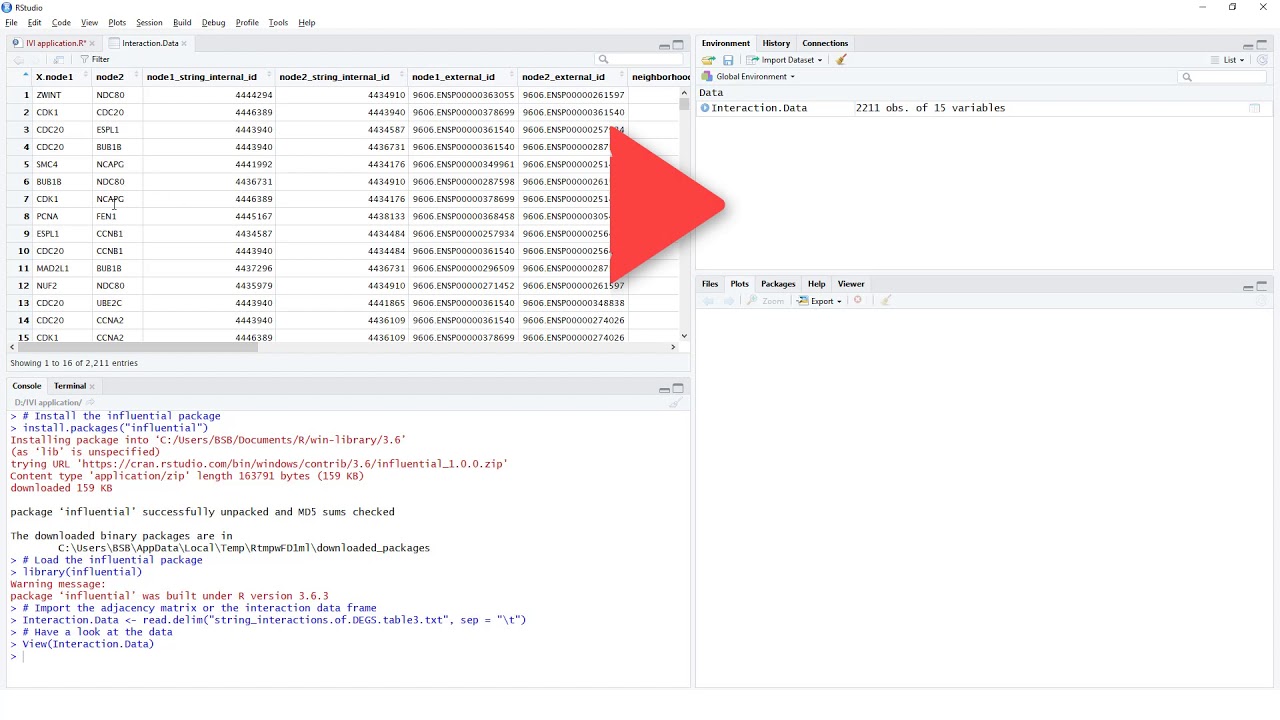
The following tutorial video demonstrates how to simply calculate the IVI value of
all of the nodes within a network.
 ## Network visualization {#NetVis}
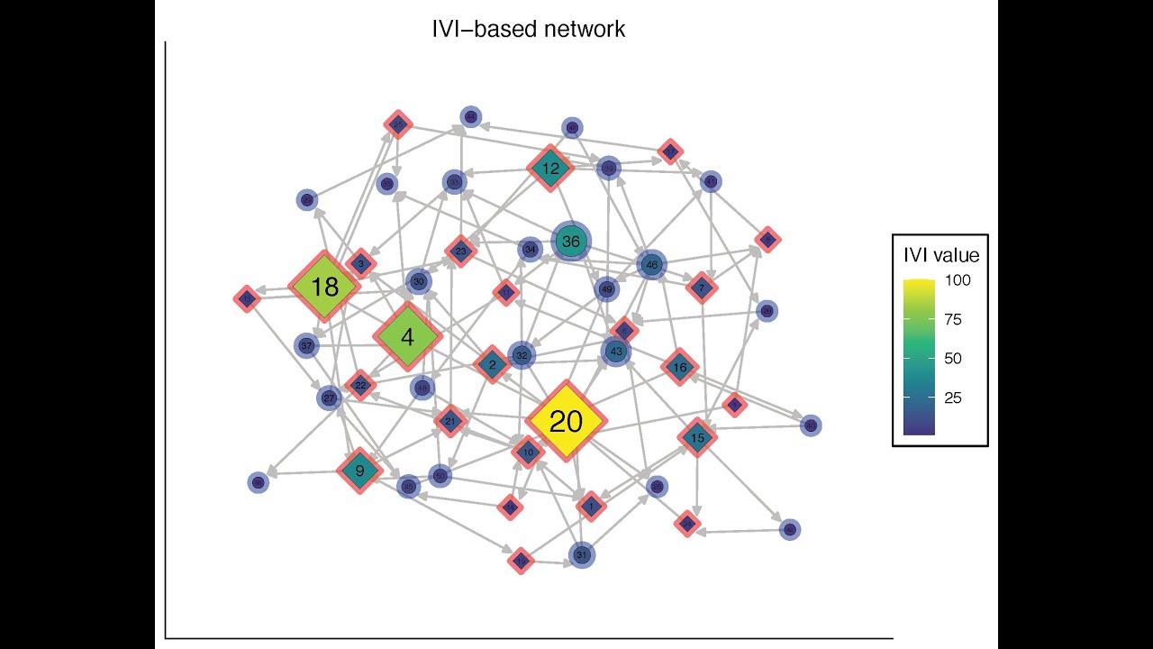
The `cent_network.vis` is a function for the visualization of a network based on applying a centrality measure to the size and color of network nodes. The centrality of network nodes could be calculated by any means and based on any centrality index. Here, we demonstrate the visualization of a network according to [IVI](#IVI) values.
```{r net.for.vis, eval=FALSE}
# Reconstructing the graph
set.seed(70)
My_graph <- igraph::sample_gnm(n = 50, m = 120, directed = TRUE)
# Calculating the IVI values
My_graph_IVI <- ivi(My_graph, directed = TRUE)
# Visualizing the graph based on IVI values
My_graph_IVI_Vis <- cent_network.vis(graph = My_graph,
cent.metric = My_graph_IVI,
directed = TRUE,
plot.title = "IVI-based Network",
legend.title = "IVI value")
My_graph_IVI_Vis
```

The above figure illustrates a simple use case of the function `cent_network.vis`. You can apply this function to directed/undirected and/or weighted/unweighted networks. Also, a complete flexibility (list of arguments) have been provided for the adjustment of colors, transparencies, sizes, titles, etc. Additionally, several different layouts have been provided that could be conveniently applied to a network.
## Network visualization {#NetVis}
The `cent_network.vis` is a function for the visualization of a network based on applying a centrality measure to the size and color of network nodes. The centrality of network nodes could be calculated by any means and based on any centrality index. Here, we demonstrate the visualization of a network according to [IVI](#IVI) values.
```{r net.for.vis, eval=FALSE}
# Reconstructing the graph
set.seed(70)
My_graph <- igraph::sample_gnm(n = 50, m = 120, directed = TRUE)
# Calculating the IVI values
My_graph_IVI <- ivi(My_graph, directed = TRUE)
# Visualizing the graph based on IVI values
My_graph_IVI_Vis <- cent_network.vis(graph = My_graph,
cent.metric = My_graph_IVI,
directed = TRUE,
plot.title = "IVI-based Network",
legend.title = "IVI value")
My_graph_IVI_Vis
```

The above figure illustrates a simple use case of the function `cent_network.vis`. You can apply this function to directed/undirected and/or weighted/unweighted networks. Also, a complete flexibility (list of arguments) have been provided for the adjustment of colors, transparencies, sizes, titles, etc. Additionally, several different layouts have been provided that could be conveniently applied to a network.
Tip: For highly crowded networks, the "grid" layout is often the most appropriate choice.
The following tutorial video demonstrates how to visualize a network based on the centrality of nodes (e.g. their `IVI` values).
 ## IVI shiny app {#IVIShiny}
Interactive app
Explore IVI without writing a full analysis script
Launch the bundled Shiny app for IVI calculation and IVI-based network visualization:
influential::runShinyApp("IVI")
You can also use the Influential Software Package server.
Back to top ↑
# Identification of the most important network spreaders {#SpreadingScore}
Information spreading
Spreading score
Integrates complementary centrality measures to prioritize nodes with high potential to spread information throughout a network.
Sometimes we seek to identify not necessarily the most influential nodes but nodes
with the greatest potential in spreading of information throughout the network.
**Spreading score**
: `spreading.score` is an integrative score made up of four different centrality measures
including ClusterRank, neighborhood connectivity, betweenness centrality, and
collective influence. Also, Spreading score reflects the spreading potential of
each node within a network and is one of the major components of the [`IVI`](#IVI).
```{r Spreading.score, eval=FALSE}
# Preparing the data
MyData <- coexpression.data
# Reconstructing the graph
My_graph <- graph_from_data_frame(MyData)
# Extracting the vertices
GraphVertices <- V(My_graph)
# Calculation of Spreading score
Spreading.score <- spreading.score(graph = My_graph,
vertices = GraphVertices,
weights = NULL, directed = FALSE, mode = "all",
loops = TRUE, d = 3, scale = "range")
head(Spreading.score)
#> ADAMTS9-AS2 C8orf34-AS1 CADM3-AS1 FAM83A-AS1 FENDRR LANCL1-AS1
#> 42.932497 38.094111 45.114648 1.587262 100.000000 49.193292
```
Spreading score could be also calculated for *directed* and/or *weighted* graphs via specifying the `directed`, `mode`, and `weights` parameters. The results could be conveniently illustrated using the [centrality-based network visualization function](#NetVis).
Back to top ↑
# Identification of the most important network hubs {#HubnessScore}
Local network power
Hubness score
Summarizes local topological strength using degree centrality and local H-index.
In some cases, the goal is to identify nodes with the strongest influence within their surrounding local environments.
**Hubness score**
: `hubness.score` is an integrative score made up of two different centrality measures
including degree centrality and local H-index. Also, Hubness score reflects the power
of each node in its surrounding environment and is one of the major components of the [`IVI`](#IVI).
```{r Hubness.score, eval=FALSE}
# Preparing the data
MyData <- coexpression.data
# Reconstructing the graph
My_graph <- graph_from_data_frame(MyData)
# Extracting the vertices
GraphVertices <- V(My_graph)
# Calculation of Hubness score
Hubness.score <- hubness.score(graph = My_graph,
vertices = GraphVertices,
directed = FALSE, mode = "all",
loops = TRUE, scale = "range")
head(Hubness.score)
#> ADAMTS9-AS2 C8orf34-AS1 CADM3-AS1 FAM83A-AS1 FENDRR LANCL1-AS1
#> 84.299719 46.741660 77.441514 8.437142 92.870451 88.734131
```
Hubness score can also be calculated for *directed* graphs via specifying the `directed` and `mode` parameters. The results could be conveniently illustrated using the [centrality-based network visualization function](#NetVis).
Back to top ↑
# Ranking the influence of nodes on the topology of a network based on the `SIRIR` model {#SIRIR}
Simulation-based influence
SIRIR
Uses SIR-based simulations with leave-one-out perturbation to rank nodes according to their effect on network topology and information spread.
**SIRIR**
: `SIRIR` is achieved by the integration of susceptible-infected-recovered (SIR) model with the leave-one-out cross validation technique and ranks network nodes based on their true universal influence on the network topology and spread of information. One of the applications of this function is the assessment of
performance of a novel algorithm in identification of network influential nodes.
```{r SIRIR, eval=FALSE}
# Reconstructing the graph
My_graph <- sif2igraph(Path = "Sample_SIF.sif")
# Extracting the vertices
GraphVertices <- V(My_graph)
# Calculation of influence rank
Influence.Ranks <- sirir(graph = My_graph,
vertices = GraphVertices,
beta = 0.5, gamma = 1, no.sim = 10, seed = 1234)
```
| | difference.value| rank|
|:-----|----------------:|----:|
|MRAP | 49.7| 1|
|FOXM1 | 49.5| 2|
|ATAD2 | 49.5| 2|
|POSTN | 49.4| 4|
|CDC7 | 49.3| 5|
|ZWINT | 42.1| 6|
|MKI67 | 41.9| 7|
|FN1 | 41.9| 7|
|ASPM | 41.8| 9|
|ANLN | 41.8| 9|
Back to top ↑
# Experimental data-based classification and ranking of top candidate features {#ExIR}
Experimental prioritization
ExIR
Combines experimental evidence, machine learning, network reconstruction, and integrated influence ranking to classify and prioritize candidate features.
**ExIR**
: `ExIR` is a model for the classification and ranking of top candidate features from experimental omics data. The input data can come from different experimental platforms, including transcriptomics, proteomics, bulk RNA-seq, and single-cell RNA-seq. The model combines multi-level filtration and scoring based on supervised learning, unsupervised learning, network reconstruction, and integrated influence ranking to classify and prioritize candidate features.
Depending on the input data and specified arguments, `exir` returns a graph object and one to four result tables:
+ **Drivers**: Prioritized drivers are features predicted to have the highest impact on the progression of the biological process or disease under investigation.
+ **Biomarkers**: Prioritized biomarkers are features predicted to have high sensitivity to the conditions under investigation and to the severity of those conditions.
+ **DE-mediators**: Prioritized DE-mediators are differentially expressed/abundant features that may act in a fluctuating or mediatory manner between drivers.
+ **nonDE-mediators**: Prioritized nonDE-mediators are features that are not differentially expressed/abundant but are associated with and may mediate relationships between drivers.
The `exir` function accepts experimental data in several formats, including data frames, tibbles, matrices, sparse matrices, and Seurat objects. For non-Seurat inputs, the default orientation is the common omics format, with features/genes in rows and samples/cells in columns. Internally, ExIR converts the data to the required analysis format, with samples/cells in rows and features in columns.
The `condition` argument can be either the name of a condition row/column in the input data or a character/factor vector specifying the condition of each sample/cell in the same order as the samples/cells in `Exptl_data`. For Seurat objects, `condition` should be the name of a metadata column.
## Preparing the differential/regression data
Suppose we have time-course transcriptomics data and have previously performed differential expression analysis for each step-wise comparison between time points. Suppose we have also performed regression or trajectory analysis to identify genes with significant alterations across the full time course.
```{r exir.data, eval=FALSE}
# Prepare sample feature names
gene.names <- paste("gene", 1:2000, sep = "_")
set.seed(60)
tp2.vs.tp1.DEGs <- data.frame(
logFC = rnorm(n = 700, mean = 2, sd = 4),
FDR = runif(n = 700, min = 0.0001, max = 0.049)
)
rownames(tp2.vs.tp1.DEGs) <- sample(gene.names, size = 700)
set.seed(70)
tp3.vs.tp2.DEGs <- data.frame(
logFC = rnorm(n = 1300, mean = -1, sd = 5),
FDR = runif(n = 1300, min = 0.0011, max = 0.039)
)
rownames(tp3.vs.tp2.DEGs) <- sample(gene.names, size = 1300)
set.seed(80)
regression.data <- data.frame(
R_squared = runif(n = 800, min = 0.1, max = 0.85)
)
rownames(regression.data) <- sample(gene.names, size = 800)
```
## Assembling the Diff_data
Use the function `diff_data.assembly` to automatically generate the Diff_data table for
the `ExIR` model.
```{r diff_data_assembl, eval=FALSE}
my_Diff_data <- diff_data.assembly(tp2.vs.tp1.DEGs,
tp3.vs.tp2.DEGs,
regression.data)
my_Diff_data[c(1:10),]
```
Have a look at the top 10 rows of the `Diff_data` data frame:
| | Diff_value1| Sig_value1| Diff_value2| Sig_value2| Diff_value3|
|:----------|-----------:|----------:|-----------:|----------:|-----------:|
|gene_17331 | 4.9| 0| 0| 1| 0|
|gene_12546 | 4.0| 0| 0| 1| 0|
|gene_12837 | -0.3| 0| 0| 1| 0|
|gene_18522 | 1.4| 0| 0| 1| 0|
|gene_6260 | -4.9| 0| 0| 1| 0|
|gene_2722 | -4.9| 0| 0| 1| 0|
|gene_19882 | 6.3| 0| 0| 1| 0|
|gene_2790 | 3.3| 0| 0| 1| 0|
|gene_17011 | -1.6| 0| 0| 1| 0|
|gene_8321 | 3.8| 0| 0| 1| 0|
## Preparing the experimental data (Exptl_data)
The recommended input format for non-Seurat omics data is a matrix or data frame with features in rows and samples/cells in columns. This is the default expected orientation:
```{r}
Exptl_data_orientation = "features_rows"
```
For bulk omics data, the input should usually be normalized and log-transformed before running `exir`. Alternatively, if the input is raw count-like bulk RNA-seq data, users can set:
```{r}
normalize = TRUE
```
In that case, ExIR applies TMM normalization followed by logCPM transformation using `edgeR`. This normalization strategy is suitable for many bulk RNA-seq count datasets, but users should confirm that it is appropriate for their specific data modality. If another normalization method is more appropriate, users should pre-normalize the data and keep `normalize = FALSE`.
Here, we prepare a simple normalized bulk-like expression matrix with genes in rows and samples in columns.
```{r exptl_data, eval=FALSE}
set.seed(60)
MyExptl_data <- matrix(
data = runif(n = 100000, min = 2, max = 300),
nrow = 2000,
ncol = 50,
dimnames = list(
gene.names,
c(
paste("cancer_sample", 1:25, sep = "_"),
paste("normal_sample", 1:25, sep = "_")
)
)
)
# Log-transform the data to mimic normalized log-scale bulk expression values
MyExptl_data <- log2(MyExptl_data)
MyExptl_data[1:5, c(1:5, 45:50)] %>% t()
```
Have a look at top 5 cancer and normal samples (transposed for better visualization) of the `Exptl_data`:
| | gene_1| gene_2| gene_3| gene_4| gene_5|
|:----------------|------:|------:|------:|------:|------:|
|cancer_sample_1 | 8| 8| 8| 8| 8|
|cancer_sample_2 | 7| 8| 6| 8| 8|
|cancer_sample_3 | 8| 7| 8| 7| 8|
|cancer_sample_4 | 8| 7| 7| 7| 8|
|cancer_sample_5 | 6| 4| 8| 5| 4|
|normal_sample_20 | 8| 7| 7| 8| 8|
|normal_sample_21 | 8| 7| 8| 6| 8|
|normal_sample_22 | 8| 8| 8| 7| 6|
|normal_sample_23 | 7| 6| 8| 7| 8|
|normal_sample_24 | 8| 8| 7| 5| 7|
|normal_sample_25 | 5| 7| 8| 8| 6|
When `Exptl_data_orientation = "features_columns"` The sample conditions can be supplied as a vector in the same order as the columns of MyExptl_data:
```{r condition.col, eval=FALSE}
condition <- c(rep("C", 25), rep("N", 25))
MyExptl_data$condition <- condition
```
Alternatively, if `Exptl_data_orientation = "features_rows"`, the condition can be provided as a row in the input data and the name of that row can be passed to the `condition` argument. For example:
```{r, eval=FALSE}
MyExptl_data_with_condition <- rbind(
condition = condition,
MyExptl_data
)
# In this case, condition = "condition"
```
However, for matrix-based analyses, it is generally cleaner to provide the condition as a separate vector.
## Optional pseudo-sampling for large datasets
For large datasets, especially single-cell datasets with many cells, ExIR can perform pseudo-sampling before running the main model. Pseudo-sampling is recommended when the number of samples/cells is greater than 500 or when computational resources are limited.
For bulk data, pseudo-sampling is performed within each condition group by randomly partitioning samples into non-overlapping groups and averaging normalized log-expression values within each group.
For single-cell RNA-seq data, pseudo-sampling is performed by randomly partitioning cells within each condition group, summing raw counts within each pseudo-sample, and then applying TMM normalization and logCPM transformation using `edgeR`.
The argument:
```{r}
pseudo_samples_per_group = 100
```
means that ExIR will generate 100 pseudo-samples per condition group. For example, if a condition contains 500 cells and `pseudo_samples_per_group = 100`, each pseudo-sample will contain 5 cells. If another condition contains 536 cells, 36 pseudo-samples will contain 6 cells and 64 pseudo-samples will contain 5 cells.
## Conservative feature filtering
ExIR includes an optional conservative feature-filtering step before the main RF, PCA, and correlation analyses:
```{r}
feature_filter = TRUE
```
This is not a highly variable gene filter. Instead, it removes features with insufficient prevalence, insufficient total signal if requested, or essentially zero variance. This helps reduce non-informative features before the expensive full feature-feature correlation analysis while still preserving biologically relevant non-DE mediators.
By default, features present in `Diff_data` and `Desired_list` are retained even if they fail the conservative expression/prevalence filters:
```{r}
always_keep_diff_features = TRUE
```
This helps preserve candidate differential or user-specified features while reducing uninformative background features.
## Running the `ExIR` model
Prepare the required arguments for the `exir` model.
```{r ExIR, eval=FALSE}
# The table of differential/regression data previously prepared
my_Diff_data
# Column indices of differential values in Diff_data
Diff_value <- c(1, 3)
# Column index of regression values in Diff_data
Regr_value <- 5
# Column indices of significance values in Diff_data
Sig_value <- c(2, 4)
# The matrix of normalized experimental data previously prepared
MyExptl_data
# The condition vector in the same order as the samples/columns of MyExptl_data
condition <- c(rep("C", 25), rep("N", 25))
# Optional desired list of features
set.seed(60)
MyDesired_list <- sample(gene.names, size = 500)
# Run the ExIR model
My.exir <- exir(
Desired_list = MyDesired_list,
Diff_data = my_Diff_data,
Diff_value = Diff_value,
Regr_value = Regr_value,
Sig_value = Sig_value,
Exptl_data = MyExptl_data,
Exptl_data_type = "bulk",
condition = condition,
Exptl_data_orientation = "features_rows",
normalize = FALSE,
pseudo_sample = FALSE,
feature_filter = TRUE,
cor_thresh_method = "mr",
mr = 100,
seed = 60,
verbose = FALSE
)
names(My.exir)
#> [1] "Driver table" "DE-mediator table" "Biomarker table" "Graph"
class(My.exir)
#> [1] "ExIR_Result"
```
If the input bulk RNA-seq data are raw count-like values, normalize = TRUE can be used:
```{r, eval=FALSE}
My.exir <- exir(
Desired_list = MyDesired_list,
Diff_data = my_Diff_data,
Diff_value = Diff_value,
Regr_value = Regr_value,
Sig_value = Sig_value,
Exptl_data = raw_count_matrix,
Exptl_data_type = "bulk",
condition = condition,
Exptl_data_orientation = "features_rows",
normalize = TRUE,
feature_filter = TRUE,
cor_thresh_method = "mr",
mr = 100,
seed = 60,
verbose = FALSE
)
```
The output of `exir` is an object of class `ExIR_Result`, containing a graph and one or more result tables depending on the input data and model settings.
Have a look at the output tables:
+ **Drivers**
| | Score| Z.score| Rank| P.value| P.adj|Type |
|:---------|---------:|----------:|----:|---------:|---------:|:-----------|
|gene_947 | 5.774833| -0.9620144| 286| 0.8319788| 0.8817412|Accelerator |
|gene_90 | 35.813378| 0.9440501| 54| 0.1725720| 0.8817412|Decelerator |
|gene_116 | 11.060591| -0.6266121| 221| 0.7345432| 0.8817412|Decelerator |
|gene_96 | 8.687675| -0.7771830| 248| 0.7814746| 0.8817412|Accelerator |
|gene_674 | 28.826453| 0.5007021| 77| 0.3082904| 0.8817412|Decelerator |
|gene_1017 | 24.162479| 0.2047545| 100| 0.4188820| 0.8817412|Accelerator |
********
+ **Biomarkers**
| | Score| Z.score| Rank| P.value| P.adj|Type |
|:---------|---------:|----------:|----:|----------:|---------:|:--------------|
|gene_947 | 1.000003| -0.2050551| 269| 0.58123546| 0.5812356|Up-regulated |
|gene_90 | 1.000007| -0.2050545| 246| 0.58123524| 0.5812356|Down-regulated |
|gene_116 | 1.000002| -0.2050552| 276| 0.58123549| 0.5812356|Down-regulated |
|gene_96 | 1.308484| -0.1644440| 70| 0.56530917| 0.5812356|Up-regulated |
|gene_674 | 1.017092| -0.2028053| 125| 0.58035641| 0.5812356|Down-regulated |
|gene_1017 | 12.507207| 1.3098553| 12| 0.09512239| 0.5812356|Up-regulated |
********
+ **DE-mediators**
| | Score| Z.score| Rank| P.value| P.adj|
|:---------|--------:|-----------:|----:|---------:|---------:|
|gene_592 | 11.10698| -1.01338150| 155| 0.8445610| 0.9191820|
|gene_258 | 17.95400| -0.66579750| 133| 0.7472297| 0.9191820|
|gene_549 | 55.86578| 1.25876700| 25| 0.1040573| 0.7359122|
|gene_891 | 69.81941| 1.96711288| 9| 0.0245851| 0.4578919|
|gene_1450 | 32.99729| 0.09786426| 68| 0.4610200| 0.9191820|
|gene_742 | 28.62281| -0.12420298| 79| 0.5494227| 0.9191820|
## Running exir on single-cell RNA-seq data
For single-cell RNA-seq data, raw counts are recommended when pseudo-sampling is used. The input can be a matrix, sparse matrix, or Seurat object.
For a sparse count matrix with genes in rows and cells in columns:
```{r, eval=FALSE}
My.exir.sc <- exir(
Desired_list = MyDesired_list,
Diff_data = my_Diff_data,
Diff_value = Diff_value,
Regr_value = Regr_value,
Sig_value = Sig_value,
Exptl_data = sc_counts,
Exptl_data_type = "sc",
condition = cell_condition,
Exptl_data_orientation = "features_rows",
pseudo_sample = TRUE,
pseudo_samples_per_group = 100,
feature_filter = TRUE,
cor_thresh_method = "mr",
mr = 20,
seed = 60,
verbose = FALSE
)
```
For a Seurat object:
```{r, eval=FALSE}
My.exir.seurat <- exir(
Desired_list = MyDesired_list,
Diff_data = my_Diff_data,
Diff_value = Diff_value,
Regr_value = Regr_value,
Sig_value = Sig_value,
Exptl_data = seurat_object,
Exptl_data_type = "sc",
condition = "condition",
assay = "RNA",
layer = "counts",
pseudo_sample = TRUE,
pseudo_samples_per_group = 100,
feature_filter = TRUE,
cor_thresh_method = "mr",
mr = 20,
seed = 60,
verbose = FALSE
)
```
When a Seurat object is supplied, `condition` should be the name of a metadata column. The `assay` and `layer` arguments specify which assay/layer should be used.
If single-cell data are not pseudo-sampled, users should provide appropriately normalized single-cell data and set:
```{r, eval=FALSE}
pseudo_sample = FALSE
normalize = FALSE
```
The following tutorial video demonstrates how to run the `ExIR` model on a sample experimental data.
 You can also [computationally simulate knockout and/or up-regulation](#CompManipulate) of the top candidate features outputted by ExIR to evaluate the impact of their manipulation on the flow of information/signaling and the integrity of the network prior to experimental validation.
## ExIR visualization
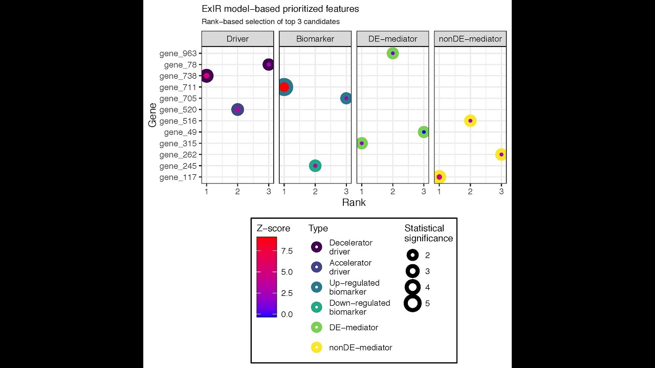
The `exir.vis` function visualizes the output of the [ExIR](#ExIR) model. The function gets the output of the ExIR model as a single argument and returns a plot of the top prioritized features of all available classes. Here, we visualize the top five candidates of the results of the `ExIR` model obtained in the previous step.
```{r exir.vis, eval=FALSE}
My.exir.Vis <- exir.vis(exir.results = My.exir,
n = 5,
y.axis.title = "Gene")
My.exir.Vis
```

A complete set of arguments is available for adjusting the visual features of the plot and selecting the desired classes, feature types, and number of top candidates.
The following tutorial video demonstrates how to visualize the results of the `ExIR` model.
You can also [computationally simulate knockout and/or up-regulation](#CompManipulate) of the top candidate features outputted by ExIR to evaluate the impact of their manipulation on the flow of information/signaling and the integrity of the network prior to experimental validation.
## ExIR visualization
The `exir.vis` function visualizes the output of the [ExIR](#ExIR) model. The function gets the output of the ExIR model as a single argument and returns a plot of the top prioritized features of all available classes. Here, we visualize the top five candidates of the results of the `ExIR` model obtained in the previous step.
```{r exir.vis, eval=FALSE}
My.exir.Vis <- exir.vis(exir.results = My.exir,
n = 5,
y.axis.title = "Gene")
My.exir.Vis
```

A complete set of arguments is available for adjusting the visual features of the plot and selecting the desired classes, feature types, and number of top candidates.
The following tutorial video demonstrates how to visualize the results of the `ExIR` model.
 ## ExIR shiny app {#ExIRShiny}
Interactive app
Run and explore ExIR interactively
The bundled Shiny app supports ExIR analysis, result visualization, and computational simulation of knockout and/or up-regulation of top candidate outputs:
influential::runShinyApp("ExIR")
You can also use the Influential Software Package server.
Back to top ↑
# Computational manipulation of cells {#CompManipulate}
In silico perturbation
Computational manipulation
Simulates feature knockout and/or up-regulation and evaluates the resulting impact on information flow within an association network.
The `comp_manipulate` is a function for the simulation of feature (gene, protein, etc.) knockout and/or up-regulation in cells.
This function works based on the [SIRIR](#SIRIR) (SIR-based Influence Ranking) model and could be applied on the output of the [ExIR](#ExIR) model or any other independent association network. For feature (gene/protein/etc.) knockout the [SIRIR](#SIRIR) model is used to remove the feature from the network and assess its impact on the flow of information (signaling) within the network.
On the other hand, in case of up-regulation a node similar to the desired node is added to the network with exactly the same connections (edges) as of the original node. Next, the [SIRIR](#SIRIR) model is used to evaluate the difference in the flow of information/signaling after adding (up-regulating) the desired feature/node compared with the original network. In case you are applying this function on the output of [ExIR](#ExIR) model, you may note that as the gene/protein knockout would impact on the integrity of the under-investigation network as well as the networks of other overlapping biological processes/pathways, it is recommended to select those features that simultaneously have the highest (most significant) [ExIR](#ExIR)-based rank and lowest knockout rank. In contrast, as the up-regulation would not affect the integrity of the network, you may select the features with highest (most significant) [ExIR](#ExIR)-based and up-regulation-based ranks. Altogether, it is recommended to select the features
with the highest (most significant) [ExIR](#ExIR)-based (major drivers or mediators of the under-investigation biological process/disease) and *Up-regulation*-based (having higher impact on the signaling within the under-investigation network when up-regulated) ranks, but with the lowest *Knockout*-based rank (having the lowest disturbance to the under-investigation as well as other overlapping networks). Below is an example of running this function on the same [ExIR](#ExIR) output generated above.
```{r comp_manipulate, eval=FALSE}
# Select which genes to knockout
set.seed(60)
ko_vertices <- sample(igraph::as_ids(V(My.exir$Graph)), size = 5)
# Select which genes to up-regulate
set.seed(1234)
upregulate_vertices <- sample(igraph::as_ids(V(My.exir$Graph)), size = 5)
Computational_manipulation <- comp_manipulate(exir_output = My.exir,
ko_vertices = ko_vertices,
upregulate_vertices = upregulate_vertices,
beta = 0.5, gamma = 1, no.sim = 100, seed = 1234)
```
Have a look at the heads of the output tables:
+ **Knockout**
| |Feature_name | Rank|Manipulation_type |
|:--|:------------|----:|:-----------------|
|2 |gene_280 | 1|Knockout |
|1 |gene_4798 | 2|Knockout |
|4 |gene_276 | 3|Knockout |
|3 |gene_16459 | 4|Knockout |
|5 |gene_7535 | 5|Knockout |
+ **Up-regulation**
|Feature_name | Rank|Manipulation_type |
|:------------|----:|:-----------------|
|gene_6433 | 1|Up-regulation |
|gene_8426 | 1|Up-regulation |
|gene_6687 | 1|Up-regulation |
|gene_1274 | 1|Up-regulation |
|gene_11555 | 1|Up-regulation |
+ **Combined**
| |Feature_name | Rank|Manipulation_type |
|:--|:------------|----:|:-----------------|
|2 |gene_280 | 1|Knockout |
|1 |gene_4798 | 2|Knockout |
|4 |gene_276 | 3|Knockout |
|3 |gene_16459 | 4|Knockout |
|11 |gene_6433 | 5|Up-regulation |
|21 |gene_8426 | 5|Up-regulation |
|31 |gene_6687 | 5|Up-regulation |
|41 |gene_1274 | 5|Up-regulation |
|51 |gene_11555 | 5|Up-regulation |
|5 |gene_7535 | 10|Knockout |
Back to top ↑
# References