Sparse generalized linear models under an exact constraint on the number of non-zero coefficients, using the Feature Selection with Annealing algorithm of Barbu, She, Ding & Gramajo (2017), IEEE TPAMI 39(2):272-286.
You tell fsa() how many variables the model may use. It
gives you exactly that many, with coefficients that carry no shrinkage
bias.
fit <- fsa(x, y, family = "gaussian", k = 10) # a 10-variable model. Not 9, not 54.## from the source tarball
install.packages("glmfsa_1.0.0.tar.gz", repos = NULL, type = "source")The package is named glmfsa rather than fsa
because CRAN already hosts an unrelated package called
FSA and CRAN names collide case-insensitively. The
fitting function is still fsa().
Start from beta = 0, then repeat: take a gradient step
on the loss, and throw away the coefficients with the smallest
magnitude, following a schedule that tightens from all M
variables down to k. Eliminated variables leave the working
design matrix entirely, so the problem shrinks as the fit proceeds.
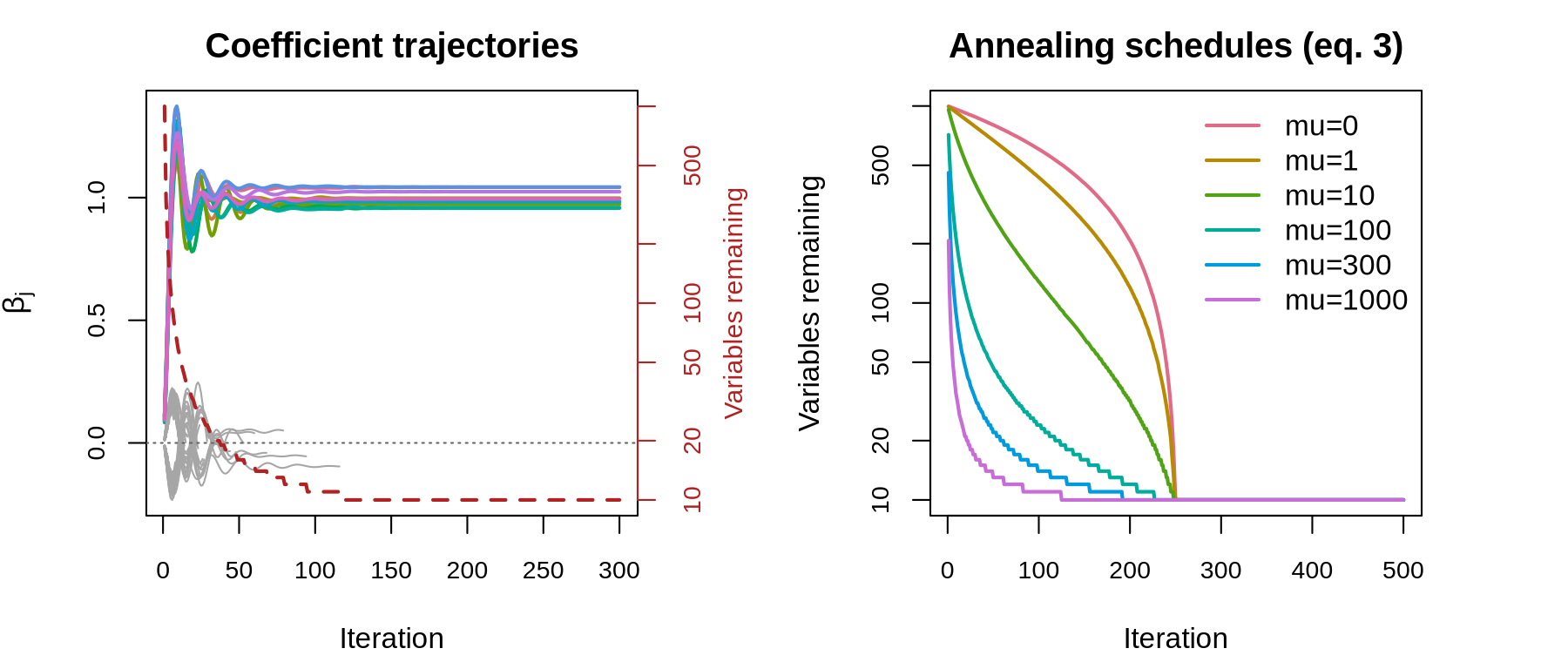
Left: every coefficient against the iteration number for a
problem with 1000 variables and 10 relevant ones; curves end as their
variables are eliminated, and the dashed red line is the number of
variables still in the model. Right: the schedule of eq. (3)
for six values of the annealing rate mu. Total work is
proportional to the area under these curves.
library(glmfsa)

set.seed(1)
n <- 300; p <- 1000
x <- matrix(rnorm(n * p), n, p)
b <- numeric(p); b[c(10, 50, 100, 200, 300)] <- 1.5
y <- as.numeric(x %*% b + rnorm(n))

fit <- fsa(x, y, k = 5)
which(coef(fit)[-1] != 0)
#> [1]  10  50 100 200 300

## a whole path of model sizes, from one annealed pass, with nested supports
path <- fsa(x, y, k = c(50, 30, 20, 12, 8, 5, 3, 2, 1))
plot(path, label = TRUE)

## choose k by cross-validation
cvfit <- cv.fsa(x, y, nfolds = 10)
coef(cvfit, k = "k.1se")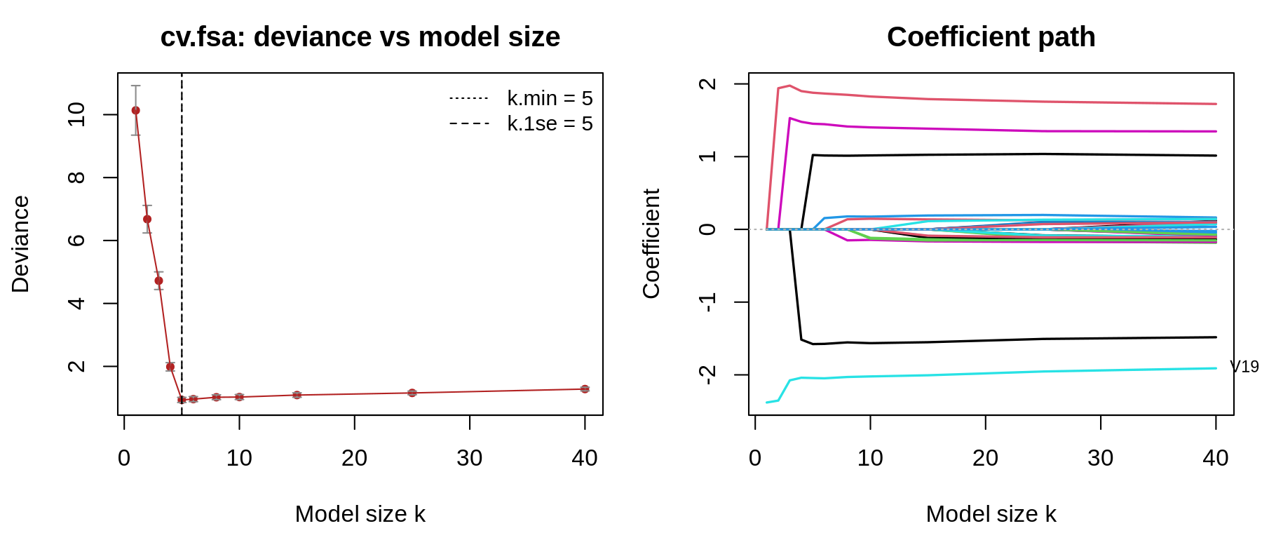
family |
Response | |
|---|---|---|
"gaussian" |
numeric | squared-error loss |
"binomial" |
2-level factor | loss = "logistic", "lorenz",
"svm", "hinge" |
"poisson" |
counts | |
"multinomial" |
K-level factor | variables selected jointly across classes |
"mgaussian" |
numeric matrix | variables selected jointly across responses |
"cox" |
Surv(time, status) |
Breslow handling of ties |
dexter ships with the package;
fetch_gisette() downloads and caches its larger
companion.
data(dexter)
dim(dexter$x)                       # 300 x 20000, sparse
cv <- cv.fsa(dexter$x, dexter$y, family = "binomial",
             k = c(100, 50, 20, 10, 5),
             s = c(0, 1e-3, 1e-2, 1e-1, 1),   # tune the ridge too
             type.measure = "class")
When p is much larger than n, pass a vector
to s and let cv.fsa() cross-validate the ridge
jointly with k. The default s = 0 is faithful
to the paper and fine when n exceeds p, but it
is not the right choice on a 300 x 20,000 design.
Dense and sparse (Matrix::dgCMatrix) designs are both
handled natively; a sparse design is never densified.
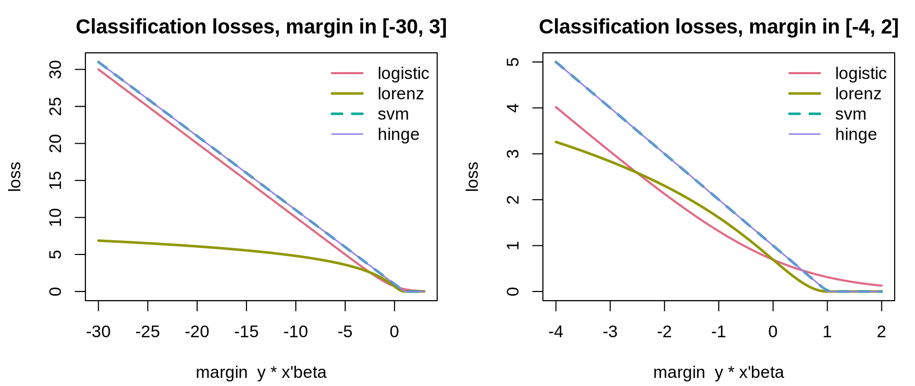
The Lorenz loss is introduced by the paper and has
no glmnet equivalent. It grows only logarithmically as the
margin becomes very negative, so a handful of mislabeled training points
cannot dominate the fit.
glmnet minimizes
loss + lambda * penalty(beta): sparsity is a consequence of
the penalty, and the model size is whatever falls out. fsa
minimizes the loss subject to ||beta||_0 <= k: sparsity
is the constraint, and you name it.
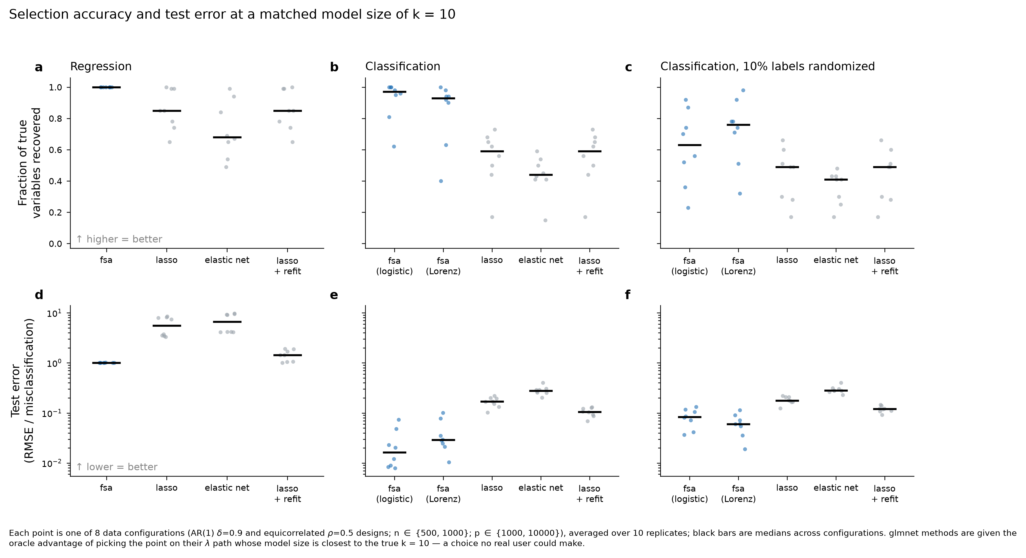
Eight data configurations – AR(1) (delta = 0.9) and
equicorrelated (rho = 0.5) designs, n in {500,
1000}, p in {1000, 10000} – ten replicates each, ten truly
relevant variables, test sets of 2000. glmnet is given the
oracle advantage of picking the point on its
lambda path whose model size is closest to the true
k = 10; a real user would have to cross-validate for
it.
Median fraction of the ten true variables recovered:
| Task | fsa | lasso | elastic net | lasso + refit |
|---|---|---|---|---|
| Regression | 1.00 | 0.85 | 0.68 | 0.85 |
| Classification | 0.97 | 0.59 | 0.44 | 0.59 |
| Classification, 10% labels randomized | 0.76 (Lorenz) | 0.49 | 0.41 | 0.49 |
Every true coefficient in the regression setting equals 1. Averaged
over the selected true variables across 20 runs at n = 500,
p = 2000, fsa returns 1.00
and the lasso at the same model size returns 0.24 – the
shrinkage that performs the selection also shrinks what it selects. This
is why refitting an unpenalized model on the selected support is
standard L1 practice; FSA needs no such step.
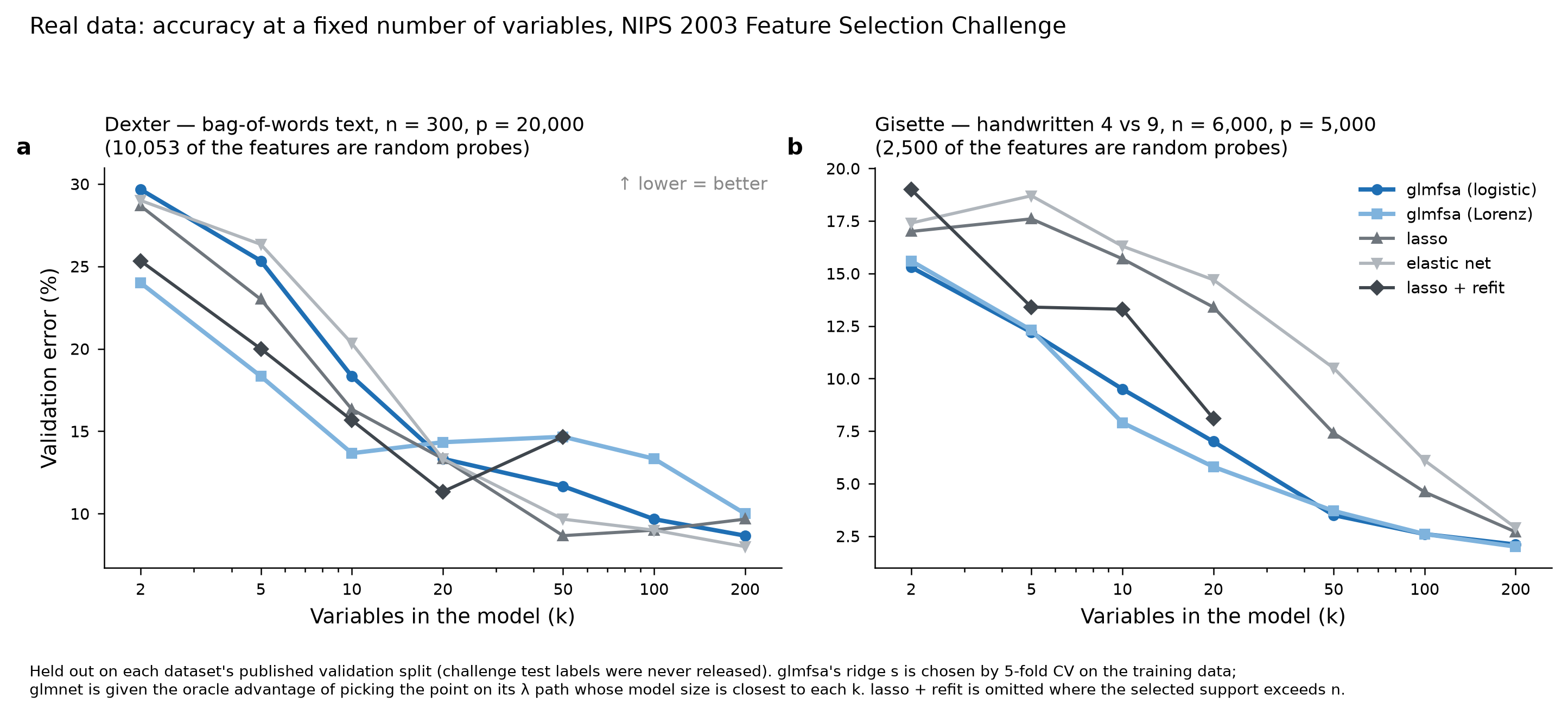
Two datasets from the NIPS 2003 Feature Selection Challenge, both
built with probes – deliberately inserted random features that
carry no signal, so selecting them is demonstrably wrong. Dexter ships
with the package; Gisette is fetched on demand with
fetch_gisette(). Evaluation is on each dataset’s published
validation split, since the challenge test labels were never released.
glmfsa’s ridge s is chosen by cross-validation
on the training data; glmnet again gets the oracle-matched
point on its lambda path.
Validation error (%) at a fixed number of variables:
| Dataset | k | glmfsa (logistic) | glmfsa (Lorenz) | lasso | elastic net |
|---|---|---|---|---|---|
| Gisette | 10 | 9.5 | 7.9 | 15.7 | 16.3 |
| Gisette | 20 | 7.0 | 5.8 | 13.4 | 14.7 |
| Gisette | 50 | 3.5 | 3.7 | 7.4 | 10.5 |
| Dexter | 5 | 25.3 | 18.3 | 23.0 | 26.3 |
| Dexter | 10 | 18.3 | 13.7 | 16.3 | 20.3 |
| Dexter | 50 | 11.7 | 14.7 | 8.7 | 9.7 |
Gisette goes to glmfsa at every model size, by a wide
margin – a 10-variable glmfsa model beats a 20-variable
lasso. Dexter is a tie that changes hands with k: the
Lorenz loss is the best option for very small models, the lasso for
larger ones. With n = 300 against 7,751 usable columns,
Dexter is the regime where shrinkage earns its keep, and it would be
dishonest to present it otherwise.
Left to choose k unaided by cross-validation, on Gisette
cv.fsa reached 1.80% with 200 variables against
cv.glmnet’s 2.30% with 263; on Dexter
cv.glmnet was slightly ahead, 9.33% with 41 variables
against 9.67% with 100.
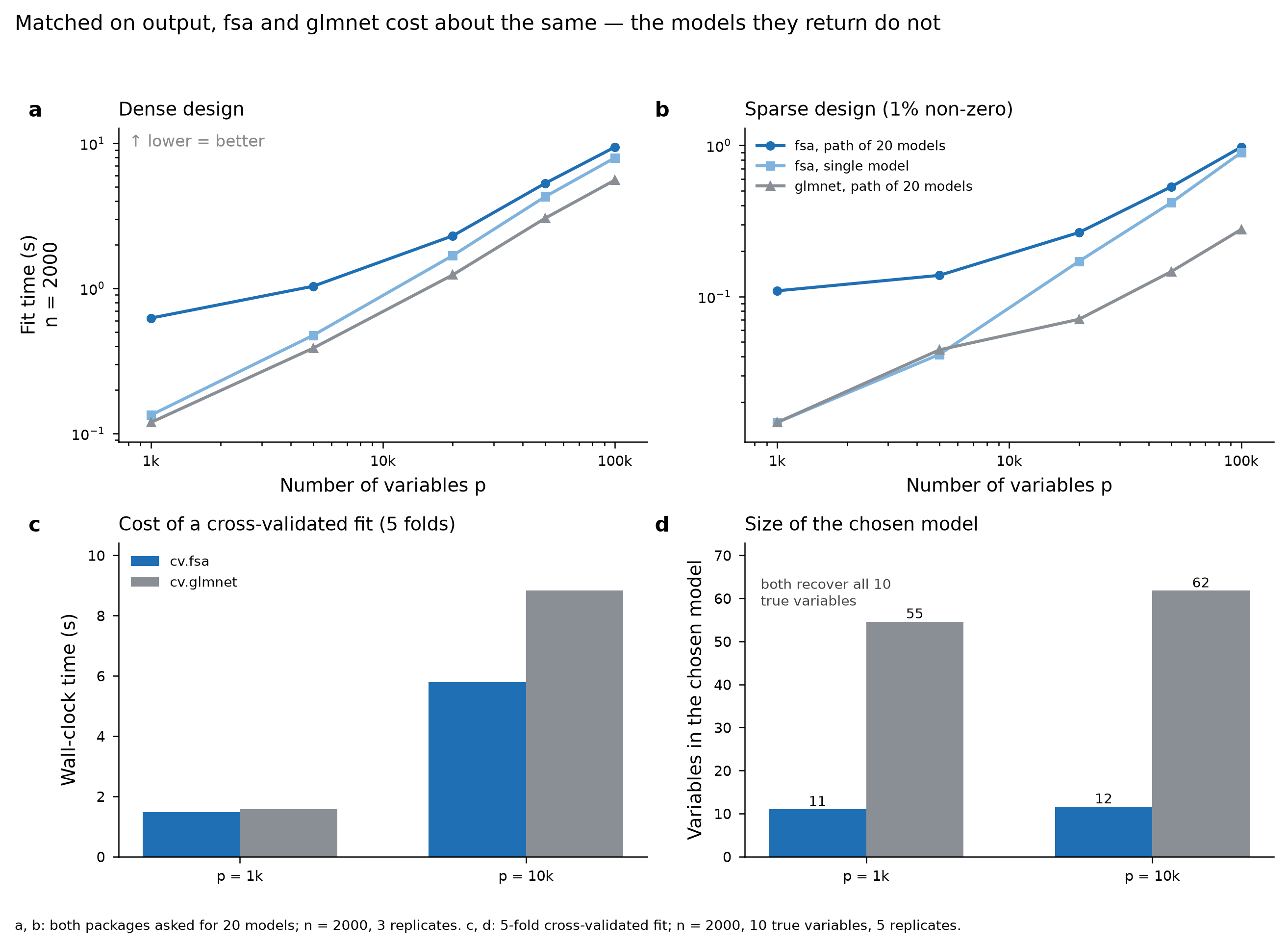
Matched on output – both packages asked for a path of 20 models – the
two are of the same order, and glmnet is several times
faster on sparse designs. Speed is not the argument for
fsa. The argument is what the time buys: in a
5-fold cross-validated fit with n = 2000 and ten true
variables, cv.fsa and cv.glmnet both recovered
all ten, but cv.glmnet needed 55-62 variables to do it
against 11-12 for cv.fsa.
If you do want speed, the annealing schedule is the dial: raising
mu and lowering niter cuts the cost directly,
and the paper’s Fig. 6 shows performance is flat over a wide range of
both.
The lasso is convex, so its path is unique and independent of initialization; FSA’s constraint set is not, and the guarantee is convergence to a local optimum with selection consistency under a slow enough schedule. On small, well-conditioned problems coordinate descent is very hard to beat, and the elastic net’s grouping of correlated predictors is often what you want. And if the goal is prediction under heavy noise rather than identifying a support, a shrunken estimator is frequently the better estimator.
| glmnet | fsa |
|---|---|
lambda |
k – the model size itself |
cv.glmnet(x, y) |
cv.fsa(x, y) |
lambda.min, lambda.1se |
k.min, k.1se |
coef(fit, s = "lambda.min") |
coef(cvfit, k = "k.min") |
penalty.factor = 0 for variable j |
include = j |
exclude = j |
exclude = j |
relax = TRUE to debias |
not needed |
vignette("glmfsa-intro") – a tour of the packagevignette("glmfsa-vs-glmnet") – the comparison above,
reproducible?fsa, ?cv.fsa, ?plot_trace,
?plot_scheduleBarbu, A., She, Y., Ding, L. and Gramajo, G. (2017). Feature Selection with Annealing for Computer Vision and Big Data Learning. IEEE Transactions on Pattern Analysis and Machine Intelligence 39(2), 272-286.
GPL-3.