kedd — Kernel Estimator and Bandwidth Selection for Density and Its Derivatives

The kedd package (v2.0.0) provides nonparametric kernel smoothing tools for R: kernel estimation of a density and of its derivatives of any order r, kernel functions, their derivatives and convolutions, and eight data-driven bandwidth selectors. Results are S4 objects with ggplot2 graphics; the \(O(n^2)\) criteria run in C++ (Rcpp) with OpenMP.

Authors: Arsalane Chouaib Guidoum (author, maintainer) and Amel Henider (author), with Iago Giné-Vázquez (contributor) — see Authors.

Features

Kernel functions (10 named kernels + the Pow(s,t) family)

Kernels with support \([-1, 1]\) are zero outside it. “r max” is the highest derivative order with \(K^{(r)} \ne 0\) (kernel.fun(), kernel.conv(), dkde()); for Pow(s,t) it is \(\min(st, 16)\) when \(s\) and \(t\) are integers and 16 otherwise. The selectors have lower limits, given in Maximum derivative order.

The power family is passed as kernel = "pow(s,t)" (or kernel.pow(s, t)) and contains uniform pow(s,0), triangular pow(1,1), Epanechnikov pow(2,1), biweight pow(2,2), triweight pow(2,3) and tricube pow(3,3). Any \(s > 0\), \(t \ge 0\) is allowed; derivatives up to order 16 are computed exactly and the constants \(\mu_2(K)\), \(\mu_4(K)\), \(R(K)\) come from Beta functions. Logistic derivatives are available up to order 20.

Bandwidth selectors

With the Gaussian and Silverman kernels every order r is allowed; with the other kernels r is limited, as given in the table Maximum derivative order r below.

All selectors return an S4 object of class bandwidth; the search interval is [0.01 * hos, 2 * hos] by default, hos being the over-smoothing bandwidth.

Maximum derivative order r

Highest deriv.order for each kernel. Above it, kernel.fun(), kernel.conv() and dkde() return zero, and the selectors return h = NA with a warning (the criterion is not finite); “—” means not available even at \(r = 0\).

For Pow(s,t), \(r^\ast\) is the largest integer \(r < t + \frac12\), with \(2r \le st\) when \(s\) and \(t\) are integers and \(r < s + \frac12\) when \(s\) is not an even integer (so pow(3,3) and tricube both give 3, 2, 1). Examples: pow(2,3) 6, 3, 2, 1; pow(2,8) 16, 6, 6, 6; pow(1.5,2.5) 16, 1, 0, —. h.scv (Gaussian kernel) has no limit and h.mlcv is for \(r = 0\) only. The same table is in ?kedd (section Maximum derivative order).

Main functions

• kernel.fun() — evaluate \(K^{(r)}(x)\) → S4 class kfun with show() and plot()
• kernel.conv() — evaluate \((K^{(r)} * K^{(r)})(x)\) → S4 class kconv
• kernel.pow(s, t) — name of a Pow(s,t) kernel, usable in every function
• dkde() — kernel density (or derivative) estimate → S4 class dkde
• All bandwidth selectors return an S4 class bandwidth with show() and plot()
• All graphics use ggplot2; lines(bw) returns a layer: plot(bw1)$plot + lines(bw2)

Installation

# Development version 2.0.0 from GitHub
# install.packages("remotes")
remotes::install_github("ac-guidoum/kedd", build_vignettes = TRUE)

# Version 2.0.0 from the source tarball
install.packages("kedd_2.0.0.tar.gz", repos = NULL, type = "source")

# or from the source directory
devtools::install("path/to/kedd_2.0.0")

# Released version on CRAN
install.packages("kedd")

Version 2.0.0 compiles C++ code: on Windows this needs Rtools.

Quick start

library(kedd)
x <- rnorm(500)

# Kernel density estimate (bandwidth chosen by UCV when h is missing)
d <- dkde(data = x, kernel = "gaussian")
plot(d)

# First derivative with its own bandwidth
h1 <- h.scv(x, deriv.order = 1)
plot(dkde(data = x, h = h1@h, deriv.order = 1))

# Bandwidth selectors
h.ucv(x)       # unbiased CV
h.bcv(x)       # biased CV
h.scv(x)       # smoothed CV (Gaussian kernel)

# Kernel function evaluation
kf <- kernel.fun(kernel = "epanechnikov", deriv.order = 1L)
plot(kf)

# Logistic and Pow(s,t) kernels
h.ucv(x, kernel = "logistic")
h.bcv(x, kernel = kernel.pow(2, 4))          # same as kernel = "pow(2,4)"
plot(kernel.fun(kernel = "pow(1.5,2.5)", deriv.order = 1L))

# Overlay two CV curves (ggplot2)
p <- plot(h.ucv(x))
p$plot + lines(h.bcv(x))

Datasets

Five samples of size 200 from the Marron & Wand (1992) normal mixtures, with known true densities (see ?"kedd-data"):

h.mcv(claw)
plot(dkde(data = bimodal, h = h.ucv(bimodal, deriv.order = 1)@h, deriv.order = 1))

Cheatsheet

A two-page summary of the package is available in cheatsheet/kedd-cheatsheet.pdf (source: cheatsheet/kedd-cheatsheet.html).

Vignette and demos

vignette("kedd", package = "kedd")   # theory, kernels, estimators, selectors, examples
demo(package = "kedd")               # list of demos
demo("kedd", package = "kedd")       # quick tour
demo("kernels", package = "kedd")    # kernels, derivatives, convolutions, Pow(s,t)
demo("bandwidths", package = "kedd") # all selectors compared on a bimodal sample

Tests

The testthat suite (≈1,460 expectations) covers every selector × kernel, the nthreads behaviour, the content of every ggplot2 figure (plot(), lines()), the datasets and input validation. It checks every kernel constant (\(\mu_2\), \(\mu_4\), \(R(K^{(r)})\)), convolution and derivative, for every kernel and every implemented order, against numerical integration, and checks Pow(s,t) against the named kernels it generalises (identical kernels, convolutions and bandwidths).

Line coverage measured with covr (tests only): 99.5 % overall.

cv <- covr::package_coverage("path/to/kedd_2.0.0", type = "tests")
covr::percent_coverage(cv)                     # 99.5
covr::report(cv)                               # line-by-line HTML report
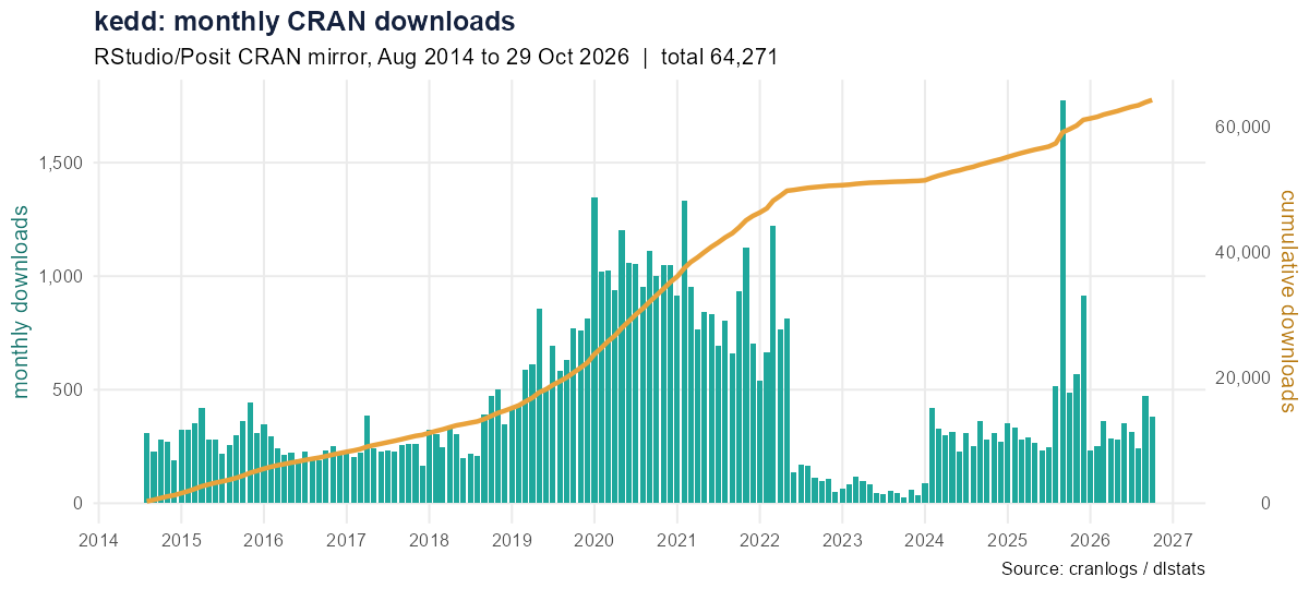
source("data-raw/benchmark.R")                 # execution time of every function

Downloads

CRAN downloads of kedd from the RStudio/Posit CRAN mirror, obtained with cranlogs (daily counts since 2014) and cross-checked with dlstats (monthly counts; identical on the 69 months both cover, Jan 2021 – Sep 2026).

* partial years (from Aug 2014; to 29 Oct 2026). The badges above are live; the figures in this section are a snapshot.

library(cranlogs)
sum(cran_downloads("kedd", from = "2014-08-01", to = Sys.Date() - 1)$count)  # total
cran_downloads("kedd", when = "last-month")

library(dlstats)
x <- cran_stats("kedd")          # monthly downloads
plot_cran_stats("kedd")

The figure and the numbers are regenerated with source("data-raw/downloads.R").

Authors

Source code: https://github.com/ac-guidoum/kedd · bug reports and suggestions: https://github.com/ac-guidoum/kedd/issues.

To cite the package (citation("kedd")):

Guidoum, A. C. (2020). Kernel estimator and bandwidth selection for density and its derivatives: the kedd package. arXiv:2012.06102. https://doi.org/10.48550/arXiv.2012.06102

References

• Bowman, A. (1984). An alternative method of cross-validation for the smoothing of kernel density estimates. Biometrika, 71, 353–360.
• Duin, R. P. W. (1976). On the choice of smoothing parameters of Parzen estimators of probability density functions. IEEE Transactions on Computers, C-25, 1175–1179.
• Feluch, W. and Koronacki, J. (1992). A note on modified cross-validation in density estimation. Computational Statistics and Data Analysis, 13, 143–151.
• Guidoum, A. C. (2020). Kernel estimator and bandwidth selection for density and its derivatives: the kedd package. arXiv:2012.06102.
• Habbema, J. D. F., Hermans, J. and Van den Broek, K. (1974). A stepwise discrimination analysis program using density estimation. Compstat 1974, Physica Verlag, Vienna.
• Hall, P., Marron, J. S. and Park, B. U. (1992). Smoothed cross-validation. Probability Theory and Related Fields, 92, 1–20.
• Jones, M. C. and Kappenman, R. F. (1991). On a class of kernel density estimate bandwidth selectors. Scandinavian Journal of Statistics, 19, 337–349.
• Marron, J. S. and Wand, M. P. (1992). Exact mean integrated squared error. The Annals of Statistics, 20, 712–736.
• Rudemo, M. (1982). Empirical choice of histograms and kernel density estimators. Scandinavian Journal of Statistics, 9, 65–78.
• Scott, D. W. and Terrell, G. R. (1987). Biased and unbiased cross-validation in density estimation. JASA, 82, 1131–1146.
• Stute, W. (1992). Modified cross validation in density estimation. Journal of Statistical Planning and Inference, 30, 293–305.
• Wand, M. P. and Jones, M. C. (1995). Kernel Smoothing. Chapman & Hall.
• Härdle, W., Marron, J. S. and Wand, M. P. (1990). Bandwidth choice for density derivatives. Journal of the Royal Statistical Society B, 52, 223–232.