This paper introduces the “damAOI” application which allows researchers to create AOIs which are at the same time locally nuanced and consistent across contexts. We use data sources on elevation, river flow, water bodies and dam construction sites to allow researchers to programmatically define their AOIs. The application was written in statistical software R and is designed to help standardize the way we consider the impacts of dams. Specifically, it programmatically determines an Area of Interest (AOI) around a dam for which impacts are measured. The previous section discusses the issues with existing approaches: bounding boxes, buffers, and basins. Our application address the issues through combining existing methods.
The software relies on openly available spatial data, specifically:
It also depends on serveral existing R packages, including:
terra, a package for working with raster data.
sf, a package for working with polygon data.
smoothr, a package to ‘smooth’ polygons.
FNN, a package for fast calculation of nearest neighbours.
shiny and leaflet, facilitating an interactive map to generate input data.
Various packages within the tidyverse for data manipulation and processing.
After preparing the input data, there are three stages to the process of creating an impacted area.
Pour points are the locations where rivers pour into and out of reservoirs. For many reservoirs, pour points can be found automatically. The pour in point(s) – where the upstream river(s) join reservoirs – typically experience the largest difference in accumulated flow, which can be computed directly from FAC hydrology data. The pour out point – the dam location – is often known. This can also be derived using the maximum FAC value of the reservoir.
For other reservoirs, pour points need to be determined by users and in our package we have developed a Shiny app which lets users select pour points using a leaflet map. This has been developed primarily for run-of-river dams, which typically see a small swelling of the river for a large distance upstream of the dam, rather than a more static lake system. This feature makes finding the pour in points automatically using FAC data impossible. The app can also help in circumstances when many rivers feed into a single reservoir, and users want to understand the upstream impacts for multiple upstream areas.
Figure @ref(fig:pourpoints) shows the pour points for Tehri dam which have been found automatically using FAC data.
Polygons of dam reservoirs are usually obtained from global georeferenced datasets. Some polygons in these datasets are inconsistent with true water extent of reservoirs, largely because of inconsistencies in the time of year that reservoir extents are measured. The first step is to adjust the polygon to match water cover of one consistent source. We suggest the CCI Global Water Bodies dataset, for larger dams the 300m2 resolution is sufficient, and the globally consistent algorithm for determining surface water extent is key.
library(terra)
library(sf)
requireNamespace("ggplot2", quietly = TRUE)
devtools::load_all()
tehri_wb <- rast(system.file("extdata", "wb_tehri.tif", package="damaoi"))
tehri_dem <- rast(system.file("extdata", "dem_tehri.tif", package="damaoi"))
tehri_adjusted <- adjustreservoirpolygon(tehri, tehri_wb, tehri_dem, 20000, 0)
ggplot2::ggplot() +
  ggplot2::geom_sf(data = tehri_adjusted, fill = "skyblue", col = "skyblue") +
  ggplot2::geom_sf(data = tehri, fill = "blue", col = "blue")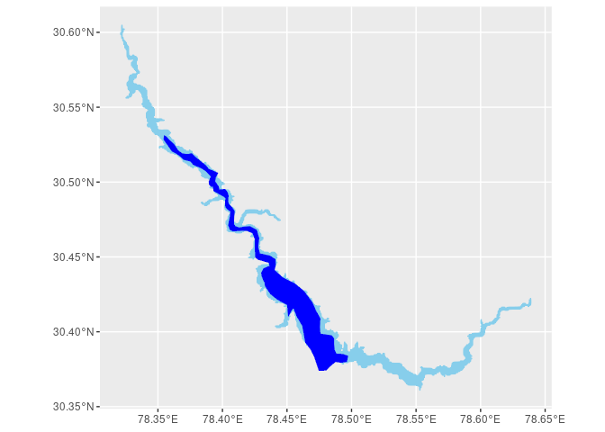
Tehri Dam is the most southerly point of the yellow polygon, which was taken directly from the GRanD dataset. To the east, there is a joining valley which was also inundated by water following the dam, but which is not included in the GRanD data. The adjustreservoirpolygon function takes three arguments, the reference polygon and the surface water raster, and ‘corrects’ the polygon. This ensures that the reservoir polygon accurately reflects the true reservoir extent following the construction of the dam.
The second stage of the process it to draw a line to follow the river downstream and upstream areas of the reservoir. Those interested in understanding downstream or upstream impacts must use these rivers, represented digitally as LINESTRINGS, to inform their impact evaluations. To map the river paths digitally, we built an algorithm using Digital Elevation Model (DEM) data and Flow ACumulation data (FAC). We recommend using HydroSHEDS 15s data as input data for the algorithm.
DEM measures the average elevation in each grid cell. FAC values are unitless, and simply measure the aggregated number of cells (in this case ~450m grid cells) that have accumulated to form the river at each cell. If a river was 200 cells long, and was joined by another 300 cells long, the flow accumulation one cell downstream of the confluence would be 501.
For the downstream river line the algorithm begins at the point in the reservoir with the highest accumulation. It searches nearby grid cells in the FAC data which are ‘water’ and selects the nearest point with a higher accumulation and a lower elevation. This is an iterative process, and continues for as far downstream as the user wishes to consider. For us, the default is 100km downstream.
For the upstream river line the algorithm begins at the point in the reservoir with the lowest accumulation. It searches nearby points which have water of a similar accumulation (to eliminate the river being diverted to insignificant upstream springs). Of these cells, it selects the nearest point with a lower accumulation and a higher elevation. This process is again repeated iteratively up to a set distance away from the reservoir.
tehri_fac <- rast(system.file("extdata", "fac_tehri.tif", package="damaoi"))
pourpoints <- autogetpourpoints(tehri_adjusted, tehri_fac)
ppid <- as.vector(1:nrow(pourpoints), mode = "list")
riverpoints <- lapply(X = ppid, FUN = getriverpoints,
                      reservoir = tehri_adjusted,
                      pourpoints = pourpoints,
                      river_distance = 100000,
                      ac_tolerance = 50,
                      e_tolerance = 10,
                      nn = 100,
                      fac = tehri_fac,
                      dem = tehri_dem)
riverpoints[sapply(riverpoints, is.null)] <- NULL
# if pour points have very small river distances flowing into them, they will be NULL elements in the list of riverpoints
# this removes the NULL values
riverlines <- pointstolines(riverpoints)

ggplot2::ggplot(tehri_adjusted) +
  ggplot2::geom_sf() +
  ggplot2::geom_sf(data = riverlines[[1]], col = "red") +
  ggplot2::geom_sf(data = riverlines[[2]], col = "blue")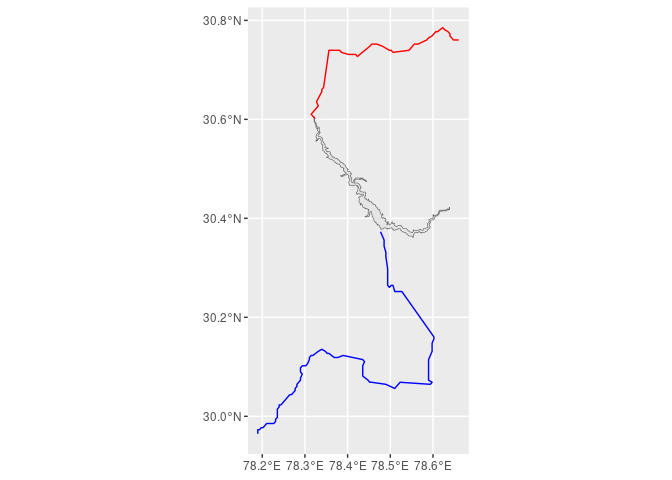
Upstream is indicated by the red line. Downstream is shown by the blue line travelling south from the reservoir towards Devprayag where there is a confluence.
The autogetpourpoints function gets pour points for the reservoir using the flow accumulation values from hydrological data. This is only possible for dams which are not ‘run of the river’ and for reservoirs with one input river.
Water bodies have a FAC value and an elevation value. The riverpoints function begins an algorithm which finds the next point in the river iteratively, searching for points downstream (upstream) which have lower (higher) elevation and a higher (lower) FAC. The river_distance parameter sets how far upstream and downstream to follow the river. The nn parameter sets the number of nearest neighbours (water bodies) to assess for these conditions. The ac_tolerance parameter sets a threshold for the point-to-point flow accumulation increase. This is so that at major confluences the algorithm will stop finding points downstream. We can see for Tehri that the downstream line is shorter than the blue line. This is because of a river confluence, where the Bhagirathi (the river running through Tehri) meets the Alakhnanda to form the Ganges. At this point, the Alakhnanda has accumulated more water than the Bhagirathi. This is a termination point for the algorithm. Any downstream effects further than this are a result of changes to both river systems, and cannot be attributed to the construction of Tehri dam. The e_tolerance parameter sets a threshold for the acceptable elevation increase if there are no points downstream (upstream) which have a lower (higher) elevation. This is important as downstream points can erroneously have a slightly higher elevation value in steep gorges because DEM values are an average across an area which can be larger than the width of rivers.
The pointstolines function converts the points and associated information generated by riverpoints to an sf linestring.
After we have drawn the river lines, we need to create a zone around the rivers and reservoir, representing how far around the rivers (and reservoir) we consider having been potentially impacted by the dam. This is in many parts a subjective choice, faced by anyone conducting spatial analysis. In our view there are a range of acceptable decisions, and some will be more appropriate in certain contexts than others. For the impacts of one dam to be compared against the impacts of a different dam, the buffer zones need to be equivalent. We set default buffers are 2km around rivers, and 5km around reservoirs.
To deal with the topography issue we then clip this buffer to the river basins. We first select the river basins which intersect the reservoir and river lines calculated in stages 1 and 2. Then we clip the buffers to these polygons.
bnb <- basinandbuffers(
  reservoir = tehri_adjusted,
  upstream = riverlines[[1]],
  downstream = riverlines[[2]],
  basins = basins_tehri,
  streambuffersize = 1500,
  reservoirbuffersize = 3000)
ggplot2::ggplot(bnb[[1]] %>% mutate(area = c("res", "down", "up"))) +
  ggplot2::geom_sf(ggplot2::aes(fill = as.factor(area)), alpha = 0.3) +
  ggplot2::geom_sf(data = bnb[[2]] %>% mutate(area = c("res", "down", "up")),
          ggplot2::aes(fill = as.factor(area))) +
  ggplot2::geom_sf(data = tehri_adjusted, fill = "grey")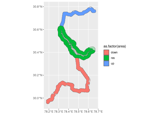
The bnb function extracts buffers for the lines and reservoir first. Second, it clips these areas by the river basins, so that areas beyond topographical barriers to water are not considered. Here shows the overlay of clipped polygons and the buffers themselves.